
Excel Formula Not Calculating - 10 Fixes
Formula not working?
Share a small sample and the result you expected.
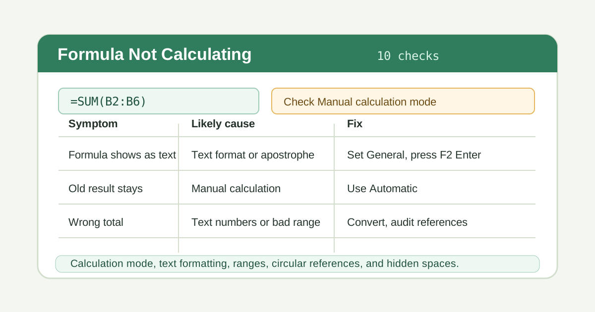
When an Excel formula is not calculating, the cause is usually one of a few practical problems: calculation mode is set to Manual, the cell is formatted as text, the formula was entered with a leading apostrophe, the referenced cells contain text instead of numbers, or the workbook has a circular reference.
Start with the quick checks below, then use the matching fix section. If your
formula is calculating but returns an error such as #VALUE!, #REF!, or
#N/A, use the broader Excel formula errors guide
after checking calculation mode.
1. Check Whether Calculation Mode Is Manual
The most common reason formulas stop updating is Manual calculation mode. In Manual mode, Excel waits until you tell it to recalculate.
Check it here:
- Go to Formulas > Calculation Options.
- Choose Automatic.
- Press
F9to recalculate the workbook.
Use this test formula in a blank cell:
=NOW()If the time does not update after you edit another cell, calculation mode is probably Manual.
| Symptom | Likely setting | Fix |
|---|---|---|
| Formula keeps an old result | Manual calculation | Set Calculation Options to Automatic |
Formula updates only after pressing F9 |
Manual calculation | Switch to Automatic |
| One workbook changes other workbooks' behavior | First opened workbook had Manual mode | Close Excel, reopen the workbook, then set Automatic |
Calculation mode is an application-level setting. A workbook opened in Manual mode can make later workbooks behave the same way during that Excel session.
2. Fix Formulas Showing as Text
If the cell displays =SUM(B2:B6) instead of the result, Excel is treating the
formula as text.
Common causes:
| Cause | What you see | Fix |
|---|---|---|
| Cell format is Text | Formula displays literally | Change format to General, then re-enter the formula |
| Leading apostrophe | '=SUM(B2:B6) in the formula bar |
Remove the apostrophe |
| Show Formulas is enabled | All formulas display on the sheet | Press Ctrl+` or turn off Formulas > Show Formulas |
After changing the cell format to General, click the formula cell, press F2,
then press Enter so Excel re-evaluates it.
Example formula that should calculate:
=SUM(B2:B6)If it still shows as text, copy the formula to Notepad, clear the cell, format the cell as General, and paste the formula back.
3. Turn Off Show Formulas
Show Formulas is useful for auditing, but it can look like every formula has stopped calculating.
Turn it off with either method:
- Press
Ctrl+`on Windows. - Or go to Formulas > Show Formulas and make sure it is not selected.
Here is the difference:
| Mode | Cell display |
|---|---|
| Normal view | 3750 |
| Show Formulas on | =SUM(B2:B6) |
This setting only changes what you see. It does not change the formula itself.
4. Convert Text Numbers to Real Numbers
A formula can calculate and still produce the wrong result if the source values are stored as text. This often happens after importing CSV files, copying data from websites, or exporting reports from other systems.
Check a value with:
=ISNUMBER(B2)If it returns FALSE, convert the text number before calculating:
=VALUE(B2)For a total, use a helper column to convert each value, then sum the converted numbers:
=SUM(C2:C10)| Original value | Test | Fix |
|---|---|---|
"125" |
=ISNUMBER(B2) returns FALSE |
=VALUE(B2) |
" 125 " |
Extra spaces | =VALUE(TRIM(B2)) |
| Imported currency text | Symbols or commas may block math | Clean the text before converting |
For a fuller cleanup workflow, see Excel Data Cleaning. For the number-specific conversion workflow, see Excel numbers stored as text.
5. Check for Hidden Spaces and Non-Printing Characters
Hidden characters can make formulas appear broken because Excel sees two values as different even when they look identical.
Use LEN to compare visible and actual length:
=LEN(A2)Clean regular extra spaces with:
=TRIM(A2)Clean non-printing characters with:
=CLEAN(A2)For non-breaking spaces copied from web pages, use:
=TRIM(SUBSTITUTE(A2,CHAR(160)," "))This is especially important before lookup formulas. If a lookup is the formula that is not calculating as expected, also review XLOOKUP troubleshooting or VLOOKUP troubleshooting.
6. Fix Circular References
A circular reference happens when a formula refers to itself, directly or indirectly. Excel may show a warning, calculate incorrectly, or keep an old value.
Example direct circular reference:
=A1+10That formula is circular if it is entered in A1.
Find circular references here:
- Go to Formulas > Error Checking.
- Choose Circular References.
- Select the listed cell.
- Rewrite the formula so it points to the intended input cell.
| Circular pattern | Example | Safer fix |
|---|---|---|
| Formula refers to its own cell | A1 contains =A1+10 |
Move the input to another cell |
| Total includes the total cell | B10 contains =SUM(B2:B10) |
Use =SUM(B2:B9) |
| Two formulas refer to each other | A1 uses B1, B1 uses A1 |
Break the dependency with a helper cell |
Only enable iterative calculation when you intentionally need a circular model, such as a finance workbook with controlled iterations.
7. Audit the Referenced Range
Sometimes the formula calculates correctly, but it points at the wrong cells. This can happen after inserting rows, copying formulas, or selecting a range too quickly.
Check the formula by selecting the cell and looking at the colored reference borders. Then confirm the start and end cells.
For example, this formula misses row 10:
=SUM(B2:B9)If the data runs through row 10, use:
=SUM(B2:B10)For growing data, convert the range to an Excel Table with Ctrl+T, then use a
structured reference:
=SUM(Table1[Amount])Tables reduce the chance that new rows are left outside the formula.
8. Lock References Before Copying Formulas
If a formula works in the first row but breaks after you fill it down, the references may be moving when they should stay fixed.
Example tax calculation:
=B2*$F$1Here, B2 should change by row, but $F$1 should stay locked as the tax rate.
| Reference | Filled down from row 2 | Use when |
|---|---|---|
B2 |
Becomes B3, B4, B5 |
Each row has its own input |
$F$1 |
Stays $F$1 |
Every row uses the same rate or assumption |
$A$2:$D$100 |
Range stays fixed | Lookup tables and source ranges |
For more examples, see Excel cell references. If you are using the fill handle to copy formulas quickly, pair this with Autofill options in Excel.
9. Check for Formula Errors Hidden by IFERROR
IFERROR is useful for clean reports, but it can hide the real reason a formula
is not working.
This formula hides every error:
=IFERROR(VLOOKUP(A2,$F$2:$G$100,2,FALSE),"")During debugging, temporarily remove IFERROR:
=VLOOKUP(A2,$F$2:$G$100,2,FALSE)Then fix the actual error. For lookup-specific errors, use How to Fix VLOOKUP #N/A in Excel or the Excel XLOOKUP tutorial.
| Hidden result | Possible real error | What to check |
|---|---|---|
| Blank cell | #N/A |
Missing lookup value or text-number mismatch |
| Blank cell | #VALUE! |
Wrong data type or mismatched ranges |
| Blank cell | #REF! |
Deleted reference or invalid column index |
Use IFERROR again only after you understand which errors are expected.
10. Recalculate, Save, and Test a Simple Formula
After fixing the likely cause, force Excel to recalculate and test a simple formula in a blank area.
Useful recalculation shortcuts:
| Shortcut | Action |
|---|---|
F9 |
Recalculate all open workbooks |
Shift+F9 |
Recalculate the active worksheet |
Ctrl+Alt+F9 |
Force a full recalculation |
Use this small test table:
| Cell | Value |
|---|---|
| A2 | 10 |
| A3 | 20 |
| A4 | 30 |
Test formula:
=SUM(A2:A4)Expected result:
| Formula | Result |
|---|---|
=SUM(A2:A4) |
60 |
If this simple formula works but your real formula does not, the problem is in the real formula's references, source data, or function logic.
11. Quick Troubleshooting Checklist
Use this order when a formula is not calculating:
- Set Formulas > Calculation Options to Automatic.
- Turn off Show Formulas.
- Change formula cells from Text to General, then re-enter them.
- Remove leading apostrophes before formulas.
- Convert text numbers with
VALUEor Text to Columns. - Clean hidden spaces with
TRIM,CLEAN, orSUBSTITUTE. - Check for circular references.
- Confirm the referenced range includes the right rows and columns.
- Lock fixed references before copying formulas.
- Remove
IFERRORtemporarily so real errors are visible.
12. Related Guides
- Decode
#VALUE!,#REF!,#N/A, and other problems with Excel formula errors. - Learn how references move when formulas are copied in Excel cell references.
- Clean imported numbers, spaces, and hidden characters with Excel Data Cleaning.
- Convert numeric-looking values with Excel numbers stored as text.
- Use Autofill options in Excel after locking references correctly.
- Fix lookup-specific failures with XLOOKUP troubleshooting or VLOOKUP troubleshooting.
- Use LET in Excel to make long formulas easier to debug.
13. Summary
Most formulas that are not calculating can be fixed without rebuilding the workbook. Start with calculation mode, Show Formulas, and text formatting. Then check source data, circular references, copied references, and hidden errors.
Once a simple SUM formula calculates correctly, work outward: verify the real
formula's inputs, ranges, and expected result one piece at a time.
Need help fixing a formula?
Share the formula, a small sample table, and the result you expected. This free beta helps us learn which Excel problems readers actually need solved.
Ask for formula help