Excel Formula Errors: A Complete Guide to Fixing #N/A, #REF!, #VALUE! & More

We’ve all been there: you spend minutes crafting an Excel formula, hit Enter, and—boom—a weird code like #N/A or #REF! pops up instead of your result. Frustrating, right? But here’s the good news: these errors aren’t random. They’re Excel’s way of telling you exactly what’s wrong—and how to fix it.

In this guide, we’ll break down every common Excel formula error, explain why it happens, and show you step-by-step solutions with real examples. By the end, you’ll turn those red error messages into working formulas in no time.

1. #N/A Error: "Not Available"

What It Means

Excel can’t find the data your formula is looking for. This is super common with lookup functions like VLOOKUP, INDEX-MATCH, or HLOOKUP.

Why It Happens

• You’re using VLOOKUP to find a value that doesn’t exist in the lookup range (e.g., searching for "Laptop" in a list that only has "Phone" and "Tablet").
• Your data range is incomplete (e.g., your VLOOKUP references A1:A10, but the value you need is in A11).
• You’re referencing an empty cell or a cell with no matching data.

How to Fix It

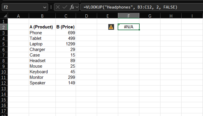
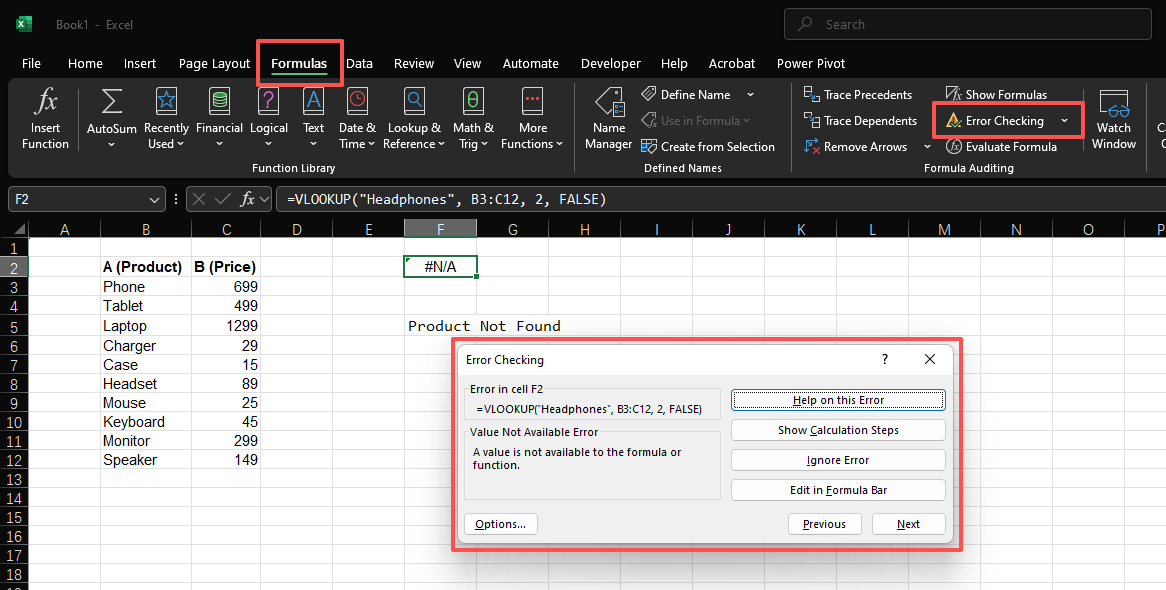
Let’s use a VLOOKUP example to fix this. Suppose you have a product list (A2:B10) and want to find the price of "Headphones" with:
=VLOOKUP("Headphones", A2:B10, 2, FALSE)

If this returns #N/A:

1. Check the lookup value: Is "Headphones" spelled exactly (no extra spaces, lowercase/uppercase matches)?
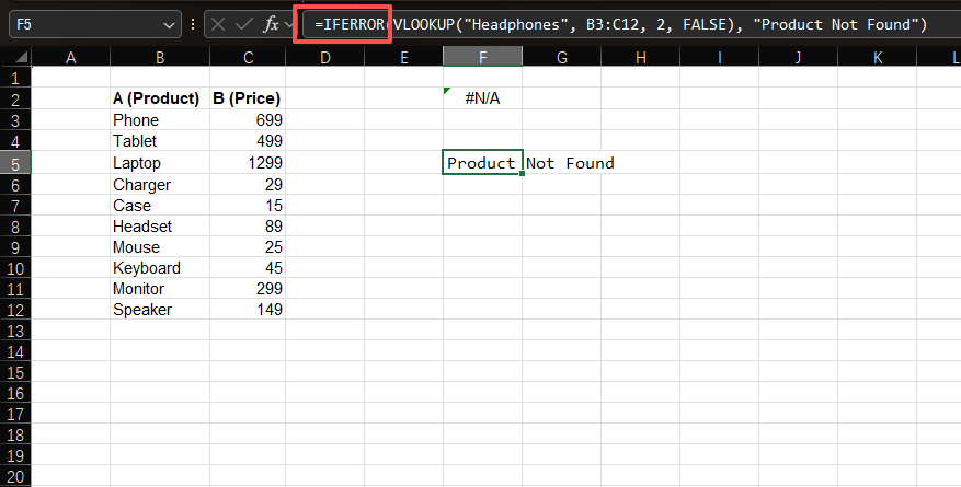
2. Expand your range: If "Headphones" is in A11, update the formula to =VLOOKUP("Headphones", A2:B11, 2, FALSE).
3. Use IFERROR for clean results: If the value might not exist (e.g., a missing product), use IFERROR to show a friendly message instead of an error:
   =IFERROR(VLOOKUP("Headphones", A2:B10, 2, FALSE), "Product Not Found")

2. #REF! Error: "Invalid Reference"

What It Means

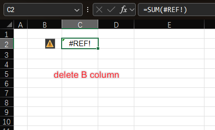
Your formula is referencing a cell, row, or column that no longer exists. Excel can’t "find" the data it needs because it’s been deleted or moved.

Why It Happens

• You deleted a column that your formula uses (e.g., your formula is =A1+B1, then you delete column B).
• You cut and pasted cells, breaking the original reference (e.g., you cut A1 and paste it over B1, which your formula references).
• You accidentally reference a cell outside Excel’s limits (e.g., =A1048577—Excel only has 1,048,576 rows).

How to Fix It

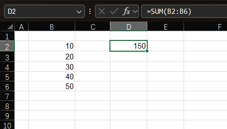
Let’s say you have a formula =SUM(A1:A5) that suddenly returns #REF!:

1. Undo recent deletions: Press Ctrl+Z to restore the deleted cell/column/row (this works if you just made the mistake).
2. Update the reference: If you deleted column A, change the formula to reference the new location (e.g., =SUM(B1:B5)).
3. Avoid cutting cells: Instead of cutting (Ctrl+X), copy (Ctrl+C) and paste—this preserves references.

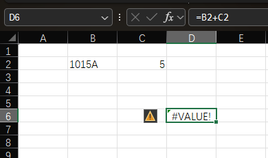
3. #VALUE! Error: "Wrong Data Type"

What It Means

Your formula is using the wrong type of data for the operation. For example, trying to add a number and text, or using a date where Excel expects a number.

Why It Happens

• You’re mixing numbers and text in a calculation (e.g., =5+"Apple"—"Apple" is text, not a number).
• A function gets the wrong input (e.g., =SUM("January", 10)—SUM needs numbers, not text).
• Your date format is broken (e.g., =DATE(2024, 13, 5)—there’s no 13th month).

How to Fix It

Let’s fix a common example: =A1+B1 where A1 is "10" (text) and B1 is 20 (number):

1. Convert text to numbers: Use the VALUE function: =VALUE(A1)+B1 (this turns "10" into 10).
2. Check for hidden spaces: Sometimes cells have invisible spaces (e.g., " 10" instead of "10"). Use TRIM to fix: =VALUE(TRIM(A1))+B1.
3. Verify function inputs: For DATE, make sure month/day are valid: =DATE(2024, 12, 5) (not 13).

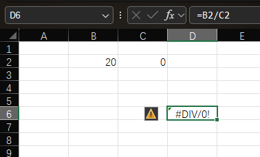
4. #DIV/0! Error: "Division by Zero"

What It Means

Your formula is trying to divide a number by 0—or by an empty cell (Excel treats empty cells as 0 in calculations).

Why It Happens

• You have a direct division by 0 (e.g., =100/0).
• You’re dividing by a cell that’s empty (e.g., =A1/B1 where B1 is blank).
• A formula result becomes 0, and you divide by it (e.g., =100/(C1-D1) where C1=D1, so C1-D1=0).

How to Fix It

Let’s use =A1/B1 where B1 might be empty or 0:

1. Use IF to check for 0: Add a condition to avoid division by 0:
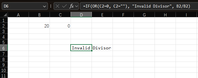
   =IF(B1=0, "Cannot Divide by 0", A1/B1)
2. Handle empty cells: If B1 could be blank, adjust the IF statement:
   =IF(OR(B1=0, B1=""), "Invalid Divisor", A1/B1)
3. Check upstream formulas: If B1 is the result of another formula (e.g., =C1-D1), fix that first to avoid 0.

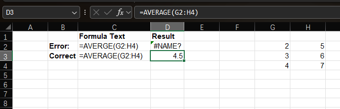
5. #NAME? Error: "Unrecognized Text"

What It Means

Excel doesn’t know what a word or phrase in your formula means. This is almost always a spelling mistake or missing quotes.

Why It Happens

• You misspelled a function name (e.g., =SUMPRODUKT(A1:A10) instead of =SUMPRODUCT(A1:A10)).
• You forgot to put text in quotes (e.g., =IF(A1>10, Over Budget, On Track) instead of =IF(A1>10, "Over Budget", "On Track")).
• You referenced a named range that doesn’t exist (e.g., =SUM(MonthlySales) but "MonthlySales" was never defined).

How to Fix It

Let’s fix a misspelled function: =AVERGE(A1:A10) (should be AVERAGE):

1. Check function spelling: Excel’s autocomplete helps—start typing the function (e.g., "AVER") and select the correct one from the list.
2. Add quotes to text: For the IF example above, update to:
   =IF(A1>10, "Over Budget", "On Track")
3. Verify named ranges: Go to the "Formulas" tab > "Defined Names" > "Name Manager" to check if your named range exists (or create it if missing).

6. #NUM! Error: "Invalid Number"

What It Means

There’s a problem with the numbers in your formula—either they’re too big/small, or the calculation is impossible.

Why It Happens

• The result is too large/small for Excel (e.g., =10^1000—Excel’s max number is ~1.797×10³⁰⁸).
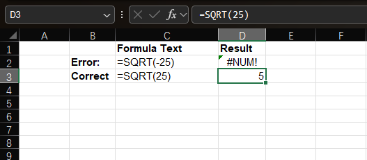
• You’re using a function with invalid numeric inputs (e.g., =SQRT(-25)—you can’t take the square root of a negative number).
• Iterative calculations (e.g., Goal Seek) don’t find a solution.

How to Fix It

Let’s fix =SQRT(-25):

1. Check for negative values: If you meant to use a positive number, update to =SQRT(25) (result: 5).
2. Adjust for large numbers: If your calculation is too big, use scientific notation (e.g., =10^300 instead of =10^1000).
3. Tweak iterative settings: Go to "File" > "Options" > "Formulas" > Check "Enable iterative calculation" to help Excel find a solution for complex formulas.

7. #NULL! Error: "No Intersection"

What It Means

You’re trying to calculate the "intersection" of two ranges that don’t overlap. This is rare, but it happens when you use a space (Excel’s intersection operator) by mistake.

Why It Happens

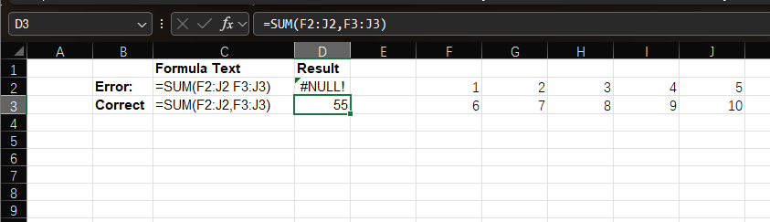
• You used a space instead of a comma or asterisk (e.g., =SUM(A1:A5 B1:B5)—you meant to add two separate ranges, not their intersection).
• The ranges you’re referencing never overlap (e.g., =A1:A3 C5:C7—these ranges are far apart, so there’s no intersection).

How to Fix It

Let’s fix =SUM(A1:A5 B1:B5):

1. Use the right operator: If you want to add both ranges, use a comma (union operator): =SUM(A1:A5, B1:B5).
2. Check range overlap: If you did want an intersection, make sure the ranges overlap (e.g., =SUM(A1:A5 A3:A7)—the intersection is A3:A5).

5 Pro Tips to Prevent Errors (Before They Happen)

1. Use Excel’s Error Checking Tool: Go to the "Formulas" tab > "Formula Auditing" > "Error Checking"—Excel will flag issues and suggest fixes.
2. Test Formulas Step-by-Step: For complex formulas (e.g., nested IFs), break them into smaller parts. Test each part in a blank cell before combining.
3. Add Data Validation: Restrict input to valid types (e.g., only numbers in a "Quantity" column). Go to "Data" > "Data Tools" > "Data Validation" to set rules.
4. Label Your Ranges: Use named ranges (e.g., "SalesData" instead of "A1:Z100")—this makes formulas easier to read and less likely to break when you move data.
5. Always Use IFERROR for Expected Errors: If a formula might return an error (e.g., a VLOOKUP for optional data), use IFERROR to keep your sheet clean (as we did in the #N/A section).

Final Thoughts

Excel errors aren’t enemies—they’re just Excel’s way of asking for help. The next time you see #N/A or #REF!, don’t panic: use this guide to identify the issue, apply the fix, and get back to analyzing your data.

Practice with the examples above, and soon you’ll be fixing errors faster than they pop up. Happy spreadsheeting!