
XLOOKUP in Excel: Formula Examples and #N/A Fixes
Formula not working?
Share a small sample and the result you expected.
XLOOKUP is the modern Excel lookup function most VLOOKUP users wish they had learned earlier. It can search one column, return a value from another column, look left or right, return multiple columns, and show a friendly message when nothing is found.
If you have ever fixed a broken VLOOKUP because the return column moved, the
lookup column was not first, or a missing value produced #N/A, XLOOKUP is a
cleaner replacement.
1. Quick Start: Write an XLOOKUP Formula
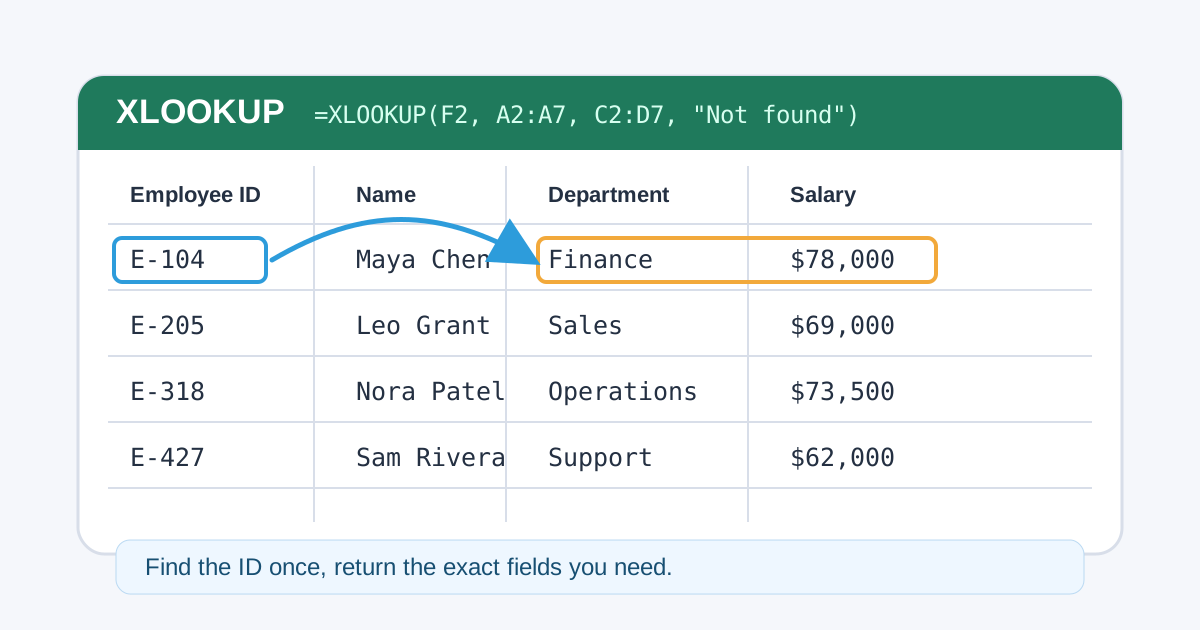
For most everyday spreadsheets, start with this pattern:
=XLOOKUP(F2, A2:A100, C2:C100, "Not found")Read it like this:
| Formula part | Meaning |
|---|---|
F2 |
The value you want to find |
A2:A100 |
The column Excel should search |
C2:C100 |
The column Excel should return from |
"Not found" |
The message to show when there is no match |
The most important XLOOKUP habit is to separate the search column from the return column. Unlike VLOOKUP, you do not count column numbers.
2. XLOOKUP Syntax
The basic syntax is:
=XLOOKUP(lookup_value, lookup_array, return_array, [if_not_found], [match_mode], [search_mode])Here is what each argument means:
| Argument | Required? | What it does |
|---|---|---|
lookup_value |
Yes | The value you want to find, such as an employee ID |
lookup_array |
Yes | The row or column Excel should search |
return_array |
Yes | The row or column Excel should return from |
[if_not_found] |
No | A custom result when no match is found |
[match_mode] |
No | Exact, approximate, or wildcard matching |
[search_mode] |
No | Search first-to-last, last-to-first, or binary search |
For most everyday spreadsheets, you only need the first four arguments:
lookup_value, lookup_array, return_array, and [if_not_found].
Microsoft's official XLOOKUP documentation notes that XLOOKUP is not available in Excel 2016 or Excel 2019. If you share workbooks with people on older Excel versions, keep that compatibility point in mind.
3. Basic Exact Match Example
Suppose you have this employee table:
| Employee ID | Name | Department | Salary |
|---|---|---|---|
| E-104 | Maya Chen | Finance | 78000 |
| E-205 | Leo Grant | Sales | 69000 |
| E-318 | Nora Patel | Operations | 73500 |
| E-427 | Sam Rivera | Support | 62000 |
If cell F2 contains an employee ID, this formula returns the matching
department:
=XLOOKUP(F2, A2:A5, C2:C5)If F2 contains E-318, the result is Operations.
This is the mental model:
| Formula part | In this example |
|---|---|
| Find this | F2 |
| Search here | A2:A5 |
| Return from here | C2:C5 |
Unlike VLOOKUP, you do not count columns. You point directly to the lookup range and the return range.
4. XLOOKUP Uses Exact Match by Default
One of the safest differences between XLOOKUP and VLOOKUP is the default match behavior.
VLOOKUP can return an approximate match if you forget the final FALSE
argument. XLOOKUP uses exact match by default.
| Function | Common exact-match formula | Risk |
|---|---|---|
| VLOOKUP | =VLOOKUP(F2, A2:D5, 3, FALSE) |
Easy to break if FALSE is omitted |
| XLOOKUP | =XLOOKUP(F2, A2:A5, C2:C5) |
Exact match is the default |
That makes XLOOKUP easier to read and less likely to return a wrong result silently.
If you need a refresher on why VLOOKUP errors happen, see the VLOOKUP troubleshooting guide. If your current problem is pulling data from another worksheet, start with VLOOKUP across sheets, then switch to XLOOKUP when your Excel version supports it.
5. Use if_not_found Instead of Showing #N/A
When a lookup value does not exist, XLOOKUP returns #N/A unless you provide
the optional [if_not_found] argument.
Instead of this:
=XLOOKUP(F2, A2:A5, C2:C5)Use this:
=XLOOKUP(F2, A2:A5, C2:C5, "Employee not found")This is cleaner than wrapping every lookup in IFNA or IFERROR.
| Employee ID entered | Result |
|---|---|
E-205 |
Sales |
E-999 |
Employee not found |
Use a custom message when the missing value is expected, such as a new employee
ID, a product code not yet loaded, or a customer that has not ordered before.
Use the raw #N/A while auditing formulas, because the error can help you spot
bad source data. If your lookup should find a match but still returns #N/A,
work through the common checks in How to Fix VLOOKUP #N/A in Excel;
the same data issues often affect XLOOKUP too. For hidden spaces and text-number
mismatches, use Excel Data Cleaning before
retrying the lookup.
For broader formula error fixes, see the Excel formula errors guide.
6. Look Left or Right Without Rearranging Columns
VLOOKUP can only look from left to right because the lookup column must be the first column in the table array. XLOOKUP does not have that limitation.
Using the same table, imagine you know the employee name in F2 and want the
employee ID from the column to the left:
=XLOOKUP(F2, B2:B5, A2:A5, "Name not found")If F2 contains Nora Patel, the formula returns E-318.
This is one of the biggest reasons to use XLOOKUP in real workbooks. You can keep your source table in a logical order instead of moving columns around just to satisfy a lookup formula.
7. Return Multiple Columns with One Formula
XLOOKUP can return more than one column when the return_array covers multiple
columns.
To return both Department and Salary for an employee ID:
=XLOOKUP(F2, A2:A5, C2:D5, "Employee not found")If F2 contains E-104, the formula spills two results:
| Department | Salary |
|---|---|
| Finance | 78000 |
This works especially well in Excel 365 because dynamic arrays can spill results into adjacent cells. Make sure the cells to the right of your formula are empty; otherwise Excel may show a spill error. For a broader explanation of spilled results, see Excel Dynamic Array Formulas.
8. Use XLOOKUP to Compare Two Columns
XLOOKUP can also help you compare two columns and mark which values are missing from another list.
Suppose column A contains product IDs from a new order file, and column D
contains product IDs from your master list. To check whether A2 exists in the
master list, use:
=XLOOKUP(A2, $D$2:$D$100, $D$2:$D$100, "Missing")If the product ID exists in column D, Excel returns the matching ID. If it does
not exist, Excel returns Missing.
For a cleaner found/missing label, wrap XLOOKUP in ISNA:
=IF(ISNA(XLOOKUP(A2, $D$2:$D$100, $D$2:$D$100)), "Missing", "Found")This is useful when checking customer lists, product IDs, invoice numbers, or any two columns that should contain matching records.
For a broader set of list comparison options, including COUNTIF, visual
highlighting, and FILTER, see
How to Compare Two Columns in Excel.
If you need two conditions to identify one row, such as Product ID plus Region, compare the modern XLOOKUP pattern with VLOOKUP with Multiple Criteria in Excel.
9. Use Match Mode Only When You Need It
For normal ID, name, SKU, or invoice lookups, leave [match_mode] blank so
XLOOKUP uses exact match.
Use match mode when you intentionally want a different behavior:
| Match mode | Meaning | Example use |
|---|---|---|
0 |
Exact match | Employee ID lookup |
-1 |
Exact match or next smaller item | Tax bracket or discount tier |
1 |
Exact match or next larger item | Minimum qualifying threshold |
2 |
Wildcard match | Partial text lookup with * or ? |
Example: return the discount rate for an order amount by finding the next smaller tier:
| Minimum Order | Discount |
|---|---|
| 0 | 0% |
| 500 | 5% |
| 1000 | 8% |
| 2500 | 12% |
=XLOOKUP(F2, A2:A5, B2:B5, "No tier", -1)If F2 is 1200, the formula returns 8%.
Approximate matches depend on how your tier table is designed. If your result looks wrong, check the sort order and confirm whether you wanted next smaller or next larger.
10. Search From Bottom to Top
By default, XLOOKUP searches from the first item to the last item. If your data
contains repeated values and you want the latest match, set [search_mode] to
-1.
Example order table:
| Customer | Order Date | Amount |
|---|---|---|
| Northwind | 2026-02-10 | 420 |
| Contoso | 2026-02-11 | 300 |
| Northwind | 2026-03-04 | 610 |
| Fabrikam | 2026-03-06 | 250 |
To return the latest amount for Northwind:
=XLOOKUP(F2, A2:A5, C2:C5, "No order found", 0, -1)The 0 keeps exact match. The -1 tells Excel to search from the bottom of the
range upward.
11. Common XLOOKUP Problems and Fixes
When XLOOKUP is not working, the cause is usually mismatched data, range sizes, or blocked spill results.
| Problem | Likely cause | Fix |
|---|---|---|
#N/A |
Lookup value is missing or has extra spaces | Check spelling, use TRIM, or add [if_not_found] |
#VALUE! |
Lookup array and return array are different sizes | Make both ranges the same height or width |
#SPILL! |
Multiple returned columns cannot spill | Clear cells where the results should appear |
| Wrong result | Approximate match mode was used incorrectly | Return to exact match or verify tier sort order |
| Works for one row but not copied rows | Relative references shifted | Use absolute references like $A$2:$A$100 |
| XLOOKUP is missing | Your Excel version may not support XLOOKUP | Use Microsoft 365, Excel 2021 or newer, or use VLOOKUP / INDEX MATCH |
| A key pasted from another sheet or website does not match | The pasted text carries a trailing space, or it is text where the column holds numbers | Rebuild the key with TRIM or VALUE before looking it up |
| The result contradicts what the filter shows | XLOOKUP searches hidden rows too, so a filtered-out row can be the match | Clear the filter while diagnosing, or use FILTER to limit the rows |
Example with absolute references:
=XLOOKUP(F2, $A$2:$A$100, $C$2:$C$100, "Not found")If your formula references move when copied, review Excel cell references before building larger lookup models.
For a focused diagnosis of #N/A, #VALUE!, #SPILL!, and copied-formula
problems, see XLOOKUP troubleshooting.
Fixing #SPILL! From a Multi-Column XLOOKUP
A #SPILL! error means XLOOKUP calculated an answer but could not write it out,
because the cells the result needs are not empty. The formula is usually correct;
the landing area is blocked.
=XLOOKUP(F2,$A$2:$A$100,$C$2:$D$100,"Not found")This returns two values, so it needs two empty cells side by side. Work through these causes in order.
| Cause | How to confirm it | Fix |
|---|---|---|
| A value, formula, or merged cell sits in the output area | Click the highlighted cell when the error appears | Clear or move the blocking cell |
| The blocking cell looks empty | A formula there returns "", which is still a value |
Select the cell and read the formula bar; it shows the formula even when the result is invisible |
| The return array covers whole columns, so far more cells want to spill | The formula uses $C:$D instead of $C$2:$D$100 |
Limit the return array to the rows you need |
| The formula sits inside an Excel Table | A table fixes how many rows a formula can occupy | Move the formula outside the table, or return a single column |
| Another spilled formula already occupies those cells | Two formulas start in the same column | Give each spilled result its own column |
If the result is a single value when you expected a block, look for an @ in front
of the ranges. Excel adds it when a formula is forced to return one value, which
stops the result from spilling at all.
When you only need one field, return a single column so nothing has to spill:
=XLOOKUP(F2,$A$2:$A$100,$C$2:$C$100,"Not found")For a dedicated spill checklist, see Excel #SPILL error causes and fixes.
XLOOKUP Returns the Wrong Row: Duplicates and Hidden Rows
Two situations make a correct XLOOKUP return a value from a row you did not expect.
The first is duplicates. XLOOKUP returns the first match unless you change the search direction, so a table with two rows for the same key looks broken when the second row is the one you wanted.
| Question | Formula | What it tells you |
|---|---|---|
| Which row is being matched? | =MATCH(F2,$A$2:$A$100,0) |
The position inside the lookup array |
| How many rows share this key? | =COUNTIF($A$2:$A$100,F2) |
Above 1 means the key is not unique |
If the key is duplicated and you want the latest row, search from the bottom with
search_mode -1:
=XLOOKUP(F2,$A$2:$A$100,$C$2:$C$100,"Not found",0,-1)The second is hidden rows. XLOOKUP searches every row in the array, including rows
hidden by a filter, so a filtered sheet can return a value that does not appear in
the visible list. Clear the filter while diagnosing, and use FILTER when the
search really should be limited to the visible rows.
If the keys themselves are duplicated in the source data, review How to Find Duplicates in Excel before building the lookup.
12. Why XLOOKUP Is Missing in Excel
If XLOOKUP is missing from your Excel formulas, the most likely reason is Excel version support. XLOOKUP is available in Microsoft 365, Excel for the web, and newer perpetual versions such as Excel 2021 and later.
If you are using Excel 2016 or Excel 2019, XLOOKUP may not be available. In that case, use one of these options:
| Need | Alternative |
|---|---|
| Simple lookup where the return column is to the right | VLOOKUP |
| Lookup left or right in older Excel | INDEX MATCH |
| Multiple criteria lookup in older Excel | INDEX MATCH with helper logic |
| A workbook shared with many Excel versions | VLOOKUP or INDEX MATCH |
For a side-by-side comparison, see VLOOKUP vs XLOOKUP vs INDEX MATCH.
13. XLOOKUP vs VLOOKUP: Quick Decision Table
Use this table when deciding which function to use:
| Situation | Better choice | Why |
|---|---|---|
| You are building a new workbook in Excel 365 or Excel 2021+ | XLOOKUP | Easier syntax and fewer lookup limitations |
| You need to look left | XLOOKUP | Return range can be anywhere |
| You need a friendly "not found" result | XLOOKUP | Built-in [if_not_found] argument |
| You need compatibility with Excel 2016 or Excel 2019 | VLOOKUP or INDEX MATCH | XLOOKUP is not available in those versions |
| You inherited an old workbook | Keep VLOOKUP if it works | Avoid unnecessary rewrites unless there is a clear problem |
For most new workbooks, XLOOKUP should be your default lookup function. Keep VLOOKUP in your toolkit for old files and compatibility requirements, but use XLOOKUP when you want formulas that are easier to read, easier to audit, and less fragile when the worksheet changes.
14. FAQ
How do I write an XLOOKUP formula in Excel?
Use this pattern:
=XLOOKUP(value_to_find, column_to_search, column_to_return, "Not found")For example, =XLOOKUP(F2, A2:A100, C2:C100, "Not found") searches for the value
in F2, looks in column A, and returns the matching value from column C.
Why is XLOOKUP missing in Excel?
Your Excel version may not support it. XLOOKUP is available in Microsoft 365, Excel for the web, Excel 2021, and newer versions. For Excel 2016 or Excel 2019, use VLOOKUP or INDEX MATCH instead.
Can XLOOKUP compare two columns?
Yes. Use one column as the lookup array and the other as the list to check. For
example, =XLOOKUP(A2, $D$2:$D$100, $D$2:$D$100, "Missing") checks whether the
value in A2 appears in column D.
Is XLOOKUP better than VLOOKUP?
For new workbooks in modern Excel, usually yes. XLOOKUP uses exact match by default, can look left or right, can return multiple columns, and avoids fragile column index numbers. VLOOKUP is still useful for older workbooks and Excel versions that do not support XLOOKUP.
15. Summary
XLOOKUP improves on VLOOKUP in several practical ways:
- It uses exact match by default
- It can return a custom result when no match is found
- It can look left or right
- It can return multiple columns
- It can search from the bottom up when you need the latest match
- It avoids column index numbers, which makes formulas easier to maintain
Start with this pattern:
=XLOOKUP(value_to_find, column_to_search, column_to_return, "Not found")Once that feels natural, add match mode and search mode only when the business case truly needs them.
16. Related Guides
- Choose between one-value lookups and dynamic row reports with Excel FILTER vs VLOOKUP.
- Compare lookup formula options in VLOOKUP vs XLOOKUP vs INDEX MATCH.
- Extract matching rows with the Excel FILTER function tutorial.
- Clean imported data before lookup checks with Excel Data Cleaning.
Need help fixing a formula?
Share the formula, a small sample table, and the result you expected. This free beta helps us learn which Excel problems readers actually need solved.
Ask for formula help