Excel Data Cleaning: How to Fix Messy Data in 5 Steps

Messy data—filled with duplicates, extra spaces, inconsistent formats, and missing values—is a top culprit behind formula errors, especially when importing from CSVs or databases. Follow these 5 structured steps to clean your data efficiently, with practical tools and a continuous real-world example.

Introduction: Why Data Cleaning Matters

When you export data from databases, CRMs, or even copy-paste from other sources, you’ll often encounter issues like:

• Unwanted duplicate rows skewing analysis
• Invisible spaces breaking VLOOKUP or sorting
• Mixed formats (e.g., dates as text, names in reverse order)
• Missing values causing #DIV/0! or #N/A errors

This tutorial uses TRIM/CLEAN functions, Data Validation, and the Text to Columns tool to resolve these problems—all demonstrated with a single "Customer Information" table that evolves through each cleaning step.

Prerequisites

• An Excel workbook with the Original Messy Data (provided below) – it includes duplicates, spaces, format chaos, and missing values
• Basic familiarity with Excel ribbon navigation

Original Messy Data (Start Here!)

Save this table in Excel as your starting point:

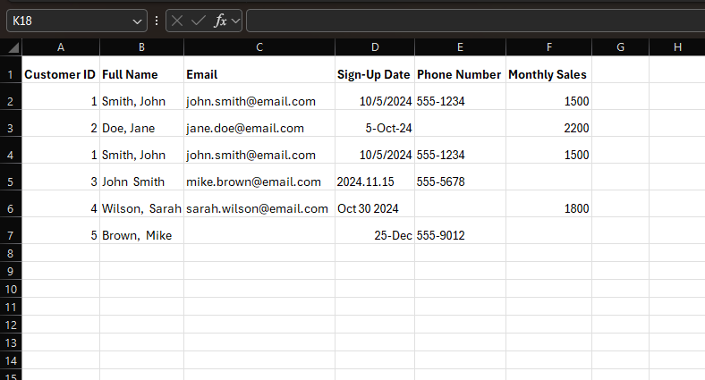
Step 1: Remove Duplicate Values

Duplicates waste space and distort results (e.g., counting Customer ID 001 twice). Excel’s built-in tool eliminates them without altering other data.

How to Do It:

1. Select your entire data range (A1:F7, including headers).
2. Go to the Data tab → Click Remove Duplicates.
3. In the pop-up: Check "My data has headers" → Select "Customer ID" (unique identifier) → Click OK.

Excel will confirm 1 duplicate row removed.

Step 2: Trim Extra Spaces with TRIM/CLEAN

Extra spaces (like the two spaces in "Brown, Mike") are invisible but break sorting and formulas. Use TRIM (for visible spaces) and CLEAN (for invisible characters) to fix this.

How to Do It:

1. In an empty column (e.g., G1), type "Cleaned Full Name" (header).
2. In G2, enter the formula: =TRIM(CLEAN(B2))
3. Press Enter → Drag the fill handle down to G6 (all rows).
4. (Optional) Copy Column G → Right-click Column B → Select Paste Values to replace the original "Full Name" column.

What It Does:

• Turns "Brown, Mike" (two spaces) into "Brown, Mike"
• Removes hidden line breaks or tabs from CSV exports

Step 3: Standardize Formats (with Data Validation)

The "Sign-Up Date" column has mixed formats (10/5/2024, 5-Oct-24, 25-Dec) that break filtering. Standardize existing dates and prevent future mess with Data Validation.

How to Standardize Existing Dates:

1. Select the "Sign-Up Date" column (D2:D6).
2. Go to the Home tab → Click the Number Format dropdown → Select "Short Date" (MM/DD/YYYY).
3. For dates that can't be standardized (like "2024.11.15"), type "N/A" (avoids text/date conflicts).

How to Prevent Future Mess (Data Validation):

1. Select empty rows for new entries (D7:D15).
2. Go to Data tab → Click Data Validation.
3. Under "Settings":
   • Allow: Date
   • Data: Between
   • Start date: 1/1/2024, End date: 12/31/2025
4. Under "Error Alert": Type "Enter a valid 2024 or 2025 date (MM/DD/YYYY)".

Step 4: Split/Merge Columns (Fix Name Chaos!)

The "Full Name" column has mixed formats: "Smith, John" (Last, First) and "John Smith" (First Last). Use Text to Columns and merge functions to standardize to "First Last".

Step 4.1: Split Names into Separate Columns

1. Select "Full Name" column (B2:B6) → Go to Data tab → Click Text to Columns.
2. Wizard Step 1: Select Delimited → Next.
3. Wizard Step 2: Check Comma (for "Last, First") and Space (for "First Last") → Next.
4. Wizard Step 3: Assign destination (C2 for Last Name, D2 for First Name) → Finish.
5. Use =TRIM(C2) and =TRIM(D2) to clean any leftover spaces.

Step 4.2: Merge to "First Last" Format

1. In Column E (header: "Standardized Name"), enter: =IF(ISNUMBER(SEARCH(",",B2)), TRIM(MID(B2,SEARCH(",",B2)+1,LEN(B2)))&" "&TRIM(LEFT(B2,SEARCH(",",B2)-1)), B2)
2. Drag the fill handle down to E6.

Result After Step 4:

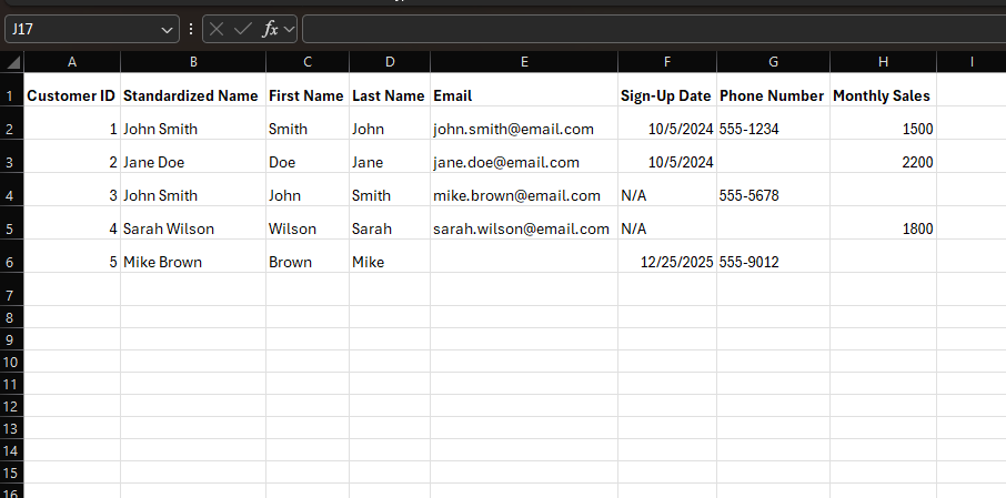
Step 5: Handle Missing Values

Blank cells (missing Phone Number, Email, Monthly Sales) break calculations. Fix them based on data type:

Option 1: Fill Text Blanks with "N/A"

For Phone Number and Email (text data):

1. Select range (F2:F6 for Phone Number, G2:G6 for Email).
2. Press Ctrl + G → Click Special → Select Blanks → OK.
3. Type N/A → Press Ctrl + Enter.

Option 2: Fill Numeric Blanks with Average

For Monthly Sales (numeric data):

1. Calculate the average of existing sales: =AVERAGE(H2:H6) (result: ~1833).
2. Select blank cells in H2:H6 → Type 1833 → Press Ctrl + Enter.

Final Clean Data Checklist

• ✅ No duplicate rows (Customer ID 001 duplicate removed)
• ✅ No extra spaces (TRIM/CLEAN fixed "Brown, Mike")
• ✅ Consistent date format (all MM/DD/YYYY or N/A)
• ✅ Standardized names (all "First Last")
• ✅ No blank cells (N/A for text, average for numbers)
• ✅ Test formulas (e.g., =SUM(H2:H6) works without errors)

Next Steps

Now that your data is clean, try:

• Creating a pivot table to summarize Monthly Sales by Customer
• Using conditional formatting to highlight sales over $2000
• Importing the cleaned table into Google Sheets or Tableau for visualization