Why Your Excel VLOOKUP Isn't Working

VLOOKUP is one of Excel's most powerful functions—when it works. But nothing is more frustrating than seeing #N/A, #VALUE!, or #REF! instead of the result you expect.

If you've ever thought, "I followed the VLOOKUP steps perfectly—why isn't it working?", you're not alone. This guide walks through the 7 most common reasons VLOOKUP fails and exactly how to fix them.

First: What VLOOKUP Actually Does (Quick Recap)

VLOOKUP searches for a value in the first column of a table and returns a matching value from a specified column. The basic formula is: =VLOOKUP(lookup_value, table_array, col_index_num, [range_lookup])

• lookup_value: What you're searching for (e.g., a product ID)
• table_array: The range of cells containing your data
• col_index_num: Which column to return data from (counting from the left)
• [range_lookup]: Use FALSE for exact matches (most common), TRUE for approximate matches

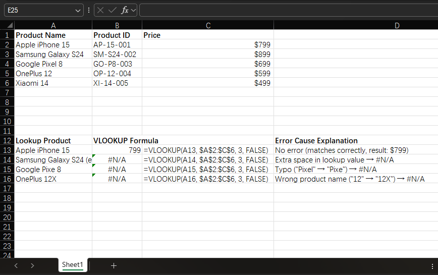
Problem 1: #N/A Error ("Not Available")

This is the most common VLOOKUP error. It means Excel can't find your lookup value in the first column of your table.

Possible Causes & Fixes:

1. Typos or extra spaces

   • Check for: Misspellings, extra spaces, or different capitalization (e.g., "apple" vs "Apple")
   • Fix: Use the TRIM function to remove extra spaces:

     =VLOOKUP(TRIM(A2), table_array, 2, FALSE)

   • Or clean your data first with Data > Text to Columns > Finish

2. Lookup value isn't in the first column

   • VLOOKUP only searches the first column of your table_array
   • Fix: Rearrange your columns so the lookup column is first, or use INDEX+MATCH instead

3. Numbers stored as text (or vice versa)

   • Check if numbers look left-aligned (text) vs right-aligned (numbers)
   • Fix: Convert text to numbers with:
     • Select column > Data > Text to Columns > Finish
     • Or use VALUE function: =VLOOKUP(VALUE(A2), table_array, 2, FALSE)

Problem 2: Incorrect Result (But No Error)

Sometimes VLOOKUP returns a value, but it's the wrong one. This is often more dangerous than an error because you might not notice it.

Common Causes:

1. Accidental approximate match

   • Forgetting to add FALSE as the last argument makes VLOOKUP return approximate matches
   • Fix: Always include FALSE for exact matches:

     =VLOOKUP(A2, B2:D100, 3, FALSE)  ✅ Correct
     =VLOOKUP(A2, B2:D100, 3)        ❌ Risky (defaults to TRUE)

2. Duplicate values in the first column

   • VLOOKUP returns the first occurrence of a value it finds
   • Fix: Remove duplicates first (see our guide on removing duplicates) or use INDEX+MATCH with COUNTIF to find all matches

3. Wrong column index number

   • col_index_num counts from the first column of your table_array, not the worksheet
   • Example: If your table is B2:D100, column 1 = B, column 2 = C, column 3 = D
   • Fix: Double-check your column count relative to your table range

Problem 3: #REF! Error ("Reference Error")

This error means Excel can't find the column you're trying to reference.

Causes & Fixes:

1. col_index_num is larger than your table has columns

   • If your table has 3 columns, using col_index_num = 4 will cause #REF!
   • Fix: Reduce your column number or expand your table_array to include more columns

2. Table_array was deleted or moved

   • If you delete columns/rows in your table range, VLOOKUP loses its reference
   • Fix: Convert your range to a named table (Ctrl+T) so references update automatically

Problem 4: #VALUE! Error

This usually happens when one of your arguments is the wrong data type.

Common Fixes:

1. col_index_num is not a number

   • Make sure you're using a number (e.g., 2) instead of text (e.g., "2" or "Column B")
   • Fix: Replace any text with a numeric value

2. table_array is not a valid range

   • Ensure your table range is entered correctly (e.g., A1:C100, not "A1-C100")
   • Fix: Click and drag to select your range instead of typing it manually

Problem 5: VLOOKUP Stops Working When You Add New Data

If your formula doesn't include new rows you add to your table:

• Fix 1: Use a dynamic named range that expands automatically
• Fix 2: Convert your data to an Excel Table (Ctrl+T) and use the table name in your formula:

  =VLOOKUP(A2, Table1, 2, FALSE)  ✅ Automatically includes new rows

Better Than VLOOKUP: Try XLOOKUP (Excel 365/2021)

If you have Excel 365 or 2021, XLOOKUP avoids most VLOOKUP problems:

• Can search in any column (not just the first)
• Doesn't return errors for missing values if you specify a default
• Easier to read syntax

Example XLOOKUP formula:=XLOOKUP(A2, B2:B100, D2:D100, "Not Found")

Quick Troubleshooting Checklist

When VLOOKUP fails, run through this list:

1. ✅ Is the lookup value in the first column of your table?
2. ✅ Did you include FALSE for exact matches?
3. ✅ Are there typos or extra spaces in your data?
4. ✅ Is col_index_num smaller than the number of columns in your table?
5. ✅ Are numbers stored as numbers (not text)?