
Excel Dynamic Array Formulas: A Complete Guide
Formula not working?
Share a small sample and the result you expected.
Dynamic array formulas changed the way modern Excel formulas work. Instead of writing one formula, copying it down, and hoping every copied reference stays correct, you can write one formula that returns many results at once.
If you use Microsoft 365 or a newer Excel version with dynamic arrays, functions
like FILTER, SORT, UNIQUE, SEQUENCE, and TEXTSPLIT can build live
lists, reports, and helper tables without manual copy-paste work.
1. Excel Version Compatibility
Dynamic arrays are available in Microsoft 365 and newer perpetual versions of Excel, but individual functions do not all have the same version support. Before sharing a workbook with other people, check which Excel version they use.
| Function group | Typical availability | Notes |
|---|---|---|
FILTER, SORT, UNIQUE, SEQUENCE |
Microsoft 365, Excel 2021+, Excel 2024 | Good starting point for most dynamic array workflows |
TEXTSPLIT |
Microsoft 365, Excel 2024 | Useful for text cleanup, but not available in older desktop versions |
TAKE |
Microsoft 365, Excel 2024 | Useful for top-N reports, but requires a newer function set |
Spill references like F2# |
Dynamic array-enabled Excel versions | Best used when the receiving workbook supports spilled arrays |
If you need to support Excel 2016 or Excel 2019, avoid relying on dynamic array formulas in shared workbooks. For those versions, use copied formulas, helper columns, Power Query, or older lookup and filter patterns instead.
2. What Is a Dynamic Array Formula?
A dynamic array formula is a formula that can return more than one value. When the result has multiple values, Excel places them into neighboring cells. This automatic expansion is called spilling.
For example, this formula creates a list of five numbers:
=SEQUENCE(5)Enter it in one cell, and Excel fills the cells below with 1, 2, 3, 4,
and 5.
| Formula | Result shape | What happens |
|---|---|---|
=SEQUENCE(5) |
5 rows by 1 column | Spills five numbers downward |
=SEQUENCE(3,4) |
3 rows by 4 columns | Spills a three-row, four-column grid |
=UNIQUE(A2:A20) |
Depends on the data | Spills only distinct values |
=FILTER(A2:D20,D2:D20>1000) |
Depends on matches | Spills every matching row |
The important idea is simple: one formula can produce a range.
3. Dynamic Arrays vs Traditional Array Formulas
Older array formulas often required Ctrl + Shift + Enter, and many users
avoided them because they felt fragile. Dynamic arrays are different: you type
the formula normally and press Enter.
| Traditional formula behavior | Dynamic array behavior |
|---|---|
| Usually returns one value per cell | Can return many values from one formula |
| Often copied down manually | Spills automatically |
| Array formulas could require special entry | Entered like a normal formula |
| Output size is usually fixed by copied formulas | Output grows or shrinks with the source data |
This matters most when your source data changes. If a filtered list has three matching rows today and twelve tomorrow, the dynamic array output can resize without rebuilding the formula.
4. Understand the Spill Range
When a formula spills, the full output range is called the spill range. Excel shows a border around the spilled result when you select the formula cell.
Suppose F2 contains:
=UNIQUE(B2:B12)If the formula returns six unique departments, the spill range might be
F2:F7.
You can refer to the entire spilled result by adding # after the first cell:
=COUNTA(F2#)That formula counts every item currently returned by the dynamic array in
F2. If the spilled list grows, F2# grows with it.
| Reference | Meaning |
|---|---|
F2 |
The first cell of the spilled formula |
F2# |
The entire current spill range from F2 |
=SUM(F2#) |
Sum all numeric values in the spilled result |
=ROWS(F2#) |
Count how many rows the spill currently has |
Spill references are useful when building dashboards, charts, validation lists, or formulas that depend on a dynamic result.
5. Create Number Lists with SEQUENCE
SEQUENCE creates a list or grid of numbers. It is useful for numbered rows,
date schedules, month labels, test data, and repeatable helper arrays.
The syntax is:
=SEQUENCE(rows, [columns], [start], [step])Examples:
| Goal | Formula |
|---|---|
| Numbers 1 through 10 | =SEQUENCE(10) |
| A 5-row, 3-column grid | =SEQUENCE(5,3) |
| Numbers 10 through 100 by tens | =SEQUENCE(10,1,10,10) |
| Next 14 dates from today | =TODAY()+SEQUENCE(14)-1 |
For a simple project schedule, this formula creates the next seven dates:
=TODAY()+SEQUENCE(7)-1Format the results as dates, and you have a live seven-day calendar that updates automatically.
6. Filter Rows with FILTER
FILTER returns only the rows or columns that meet a condition. It is one of
the most useful dynamic array functions because it replaces many manual filter,
copy, and paste workflows.
The syntax is:
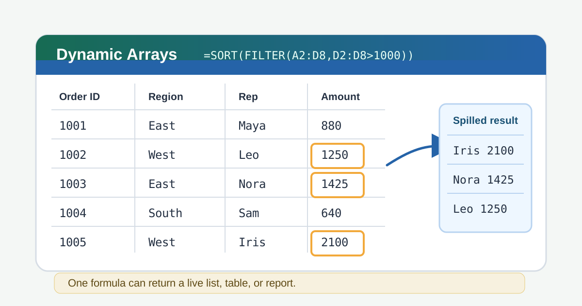
=FILTER(array, include, [if_empty])Example sales table:
| Order ID | Region | Rep | Amount |
|---|---|---|---|
| 1001 | East | Maya | 880 |
| 1002 | West | Leo | 1250 |
| 1003 | East | Nora | 1425 |
| 1004 | South | Sam | 640 |
| 1005 | West | Iris | 2100 |
To return orders where the amount is greater than 1000:
=FILTER(A2:D6, D2:D6>1000, "No matching orders")Result:
| Order ID | Region | Rep | Amount |
|---|---|---|---|
| 1002 | West | Leo | 1250 |
| 1003 | East | Nora | 1425 |
| 1005 | West | Iris | 2100 |
The condition D2:D6>1000 creates a true-or-false test for each row. FILTER
returns the rows where the test is true.
7. Filter with Multiple Conditions
For an AND condition, multiply the tests. This returns rows where both tests are true.
To return West region orders above 1000:
=FILTER(A2:D6, (B2:B6="West")*(D2:D6>1000), "No matching orders")For an OR condition, add the tests. This returns rows where at least one test is true.
To return orders from East or West:
=FILTER(A2:D6, (B2:B6="East")+(B2:B6="West"), "No matching orders")| Condition type | Pattern | Example |
|---|---|---|
| AND | (test1)*(test2) |
Region is West and amount is above 1000 |
| OR | (test1)+(test2) |
Region is East or West |
| Not equal | range<>"value" |
Region is not South |
| Blank check | range<>"" |
Cell is not blank |
If FILTER returns more rows than expected, check each condition separately in a helper column. Most mistakes come from extra spaces, mixed data types, or a condition pointing at the wrong range.
8. Get Unique Lists with UNIQUE
UNIQUE returns distinct values from a range. It is perfect for creating a
live list of departments, customers, regions, products, or categories.
Using the sales table above, this formula returns each region once:
=UNIQUE(B2:B6)Result:
| Region |
|---|
| East |
| West |
| South |
You can combine UNIQUE with SORT to create a cleaner list:
=SORT(UNIQUE(B2:B6))That pattern is especially useful for dropdown source lists. If the source data gains a new region, the unique sorted list updates automatically.
For cleaner dropdown setup, see the Excel data validation guide.
9. Sort Formula Results with SORT and SORTBY
SORT sorts a range by column number. SORTBY sorts one range by another
range. Both return dynamic arrays.
The syntax for SORT is:
=SORT(array, [sort_index], [sort_order], [by_col])To sort the sales table by Amount from largest to smallest:
=SORT(A2:D6, 4, -1)| Argument | In this example |
|---|---|
array |
A2:D6 |
sort_index |
4, because Amount is the fourth column |
sort_order |
-1, for descending order |
Use SORTBY when the sort range is easier to point at directly:
=SORTBY(A2:D6, D2:D6, -1)Both formulas produce a sorted copy of the data. They do not rearrange the original table.
For manual sorting tools and multi-column sort rules, see Excel sorting.
10. Split Text with TEXTSPLIT
TEXTSPLIT splits text into separate cells using a delimiter. It is useful
when imported data puts multiple values into one cell.
Suppose cell A2 contains:
| A |
|---|
Maya Chen | Finance | East |
This formula splits the text into columns:
=TEXTSPLIT(A2, " | ")Result:
| Name | Department | Region |
|---|---|---|
| Maya Chen | Finance | East |
You can also split by row delimiter. If a cell contains comma-separated items, this formula returns one item per row:
=TEXTSPLIT(A2,, ", ")| Original text | Formula result |
|---|---|
East, West, South |
Three spilled rows |
A-100, A-205, A-318 |
Three spilled rows |
When splitting messy imported text, clean extra spaces first with TRIM or
normalize the delimiter before splitting.
11. Combine Dynamic Array Functions
Dynamic array formulas become most powerful when you combine them. Start with a clear goal, then stack functions from the inside out.
Goal: return a sorted unique list of reps who have orders above 1000.
=SORT(UNIQUE(FILTER(C2:C6, D2:D6>1000, "")))Read it from the inside:
| Step | Formula part | What it does |
|---|---|---|
| 1 | FILTER(C2:C6, D2:D6>1000, "") |
Returns reps with orders above 1000 |
| 2 | UNIQUE(...) |
Removes duplicate rep names |
| 3 | SORT(...) |
Sorts the final list alphabetically |
Another useful pattern is a top-N report in Excel versions that support TAKE:
=TAKE(SORTBY(A2:D20, D2:D20, -1), 5)This sorts the table by Amount descending, then returns the top five rows.
If nested formulas become hard to read, use the LET function to name each
piece. See the LET function guide for that
workflow.
12. Common Dynamic Array Errors
Dynamic arrays are easier than old array formulas, but they introduce a few new things to watch.
| Error or symptom | Likely cause | Fix |
|---|---|---|
#SPILL! |
Cells in the output area are not empty | Clear the cells blocking the spill range |
#CALC! |
FILTER found no results and no [if_empty] value was provided |
Add a friendly fallback like "No results" |
| Formula returns one value only | Excel inserted implicit intersection with @ |
Remove @ if you wanted the full array |
| Result changes size unexpectedly | Source data changed | Use structured tables or leave room for the spill |
| Wrong rows are returned | Include range has a different size from array | Make the array and condition ranges the same height |
For a focused walkthrough of blocked spill ranges, merged cells, and table limitations, see Excel #SPILL error causes and fixes.
Example of a safer FILTER formula:
=FILTER(A2:D100, D2:D100>1000, "No matching orders")The third argument prevents an empty result from turning into #CALC!.
For a broader list of formula errors and fixes, see Excel formula errors.
13. Best Practices for Dynamic Array Formulas
Use these habits to keep dynamic array workbooks easy to maintain:
- Put source data in an Excel Table when possible so ranges expand cleanly
- Leave empty space below and to the right of formulas that may spill
- Use
F2#style spill references when another formula needs the full result - Add
[if_empty]to FILTER so empty results are user-friendly - Build complex formulas one function at a time before nesting them
- Avoid placing important manual data where a formula may need to spill later
If your source ranges contain many blank rows around the real data, review TRIMRANGE and trim references before building large dynamic array models.
Dynamic arrays are not only a new set of functions. They are a different way to think about worksheet design: one formula can generate the helper table, report, or list that used to require copied formulas and manual cleanup.
14. Stack, Split, and Flatten Arrays with VSTACK, HSTACK, and TOCOL
Real workbooks rarely keep everything in one range. These functions reshape arrays so the dynamic array functions above can work on a single clean input.
| Goal | Function | Example |
|---|---|---|
| Join two ranges one below the other | VSTACK |
=VSTACK(A2:C10,E2:G10) |
| Join two ranges side by side | HSTACK |
=HSTACK(A2:A10,C2:C10) |
| Turn a block into a single column | TOCOL |
=TOCOL(A2:D10,1) |
| Turn a block into a single row | TOROW |
=TOROW(A2:D10,1) |
| Remove the first row of a result | DROP |
=DROP(A2#,1) |
| Keep only the top five rows | TAKE |
=TAKE(A2#,5) |
| Keep selected columns | CHOOSECOLS |
=CHOOSECOLS(A2:D10,1,3) |
VSTACK is the one to remember for reports, because it lets you filter two
tables as if they were one:
=VSTACK(FILTER(A2:C10,C2:C10="Open","None"),FILTER(E2:G10,G2:G10="Open","None"))TOCOL flattens a rectangular block. Its second argument decides what gets
dropped: 0 keeps everything, 1 ignores blanks, 2 ignores errors, and 3
ignores both. That makes =SORT(UNIQUE(TOCOL(A2:D10,1))) a fast way to list
every distinct value in a whole block.
| Edge case | Behavior | Workaround |
|---|---|---|
VSTACK ranges have different column counts |
The narrower array is padded with #N/A |
Make both ranges the same width, or select matching columns first |
HSTACK ranges have different row counts |
The shorter array is padded with #N/A |
Match the heights, or pad deliberately with EXPAND |
Extra #N/A rows appear at the bottom of a stacked result |
Padding, not a failed lookup | Fix the source ranges, or wrap the result in IFERROR |
TOCOL on a very large block |
Every cell becomes one output row | Bound the range first, or wrap it in TRIMRANGE |
If the result is #NAME? instead of data, the function is missing from that
Excel build. VSTACK, HSTACK, TOCOL, and TOROW need Microsoft 365 or
Excel 2024, so confirm that before sharing the workbook.
15. Summary
Start with these patterns:
=FILTER(data_range, condition_range=value, "No results")
=SORT(UNIQUE(list_range))
=SEQUENCE(number_of_rows)
=TEXTSPLIT(text_cell, delimiter)
=ROWS(spill_start_cell#)
Use FILTER when you need matching rows, UNIQUE when you need a clean list,
SORT when the output should be ordered, SEQUENCE when you need generated
numbers or dates, and TEXTSPLIT when imported text needs to become columns or
rows. If you use TEXTSPLIT or TAKE, confirm that the workbook's audience has
a compatible Excel version.
Once those feel natural, combine them. A single dynamic array formula can become a live report that updates as your worksheet changes.
16. Related Guides
- Choose between dynamic row extraction and one-value lookups with Excel FILTER vs VLOOKUP.
- Extract matching rows with the Excel FILTER function tutorial.
- Compare modern lookup options with VLOOKUP vs XLOOKUP vs INDEX MATCH.
- Return multiple columns from one lookup with the Excel XLOOKUP tutorial.
- Troubleshoot blocked spill output with XLOOKUP not working.
- Manage blank edges in dynamic ranges with TRIMRANGE and trim references.
- Fix blocked dynamic array output with Excel #SPILL error causes and fixes.
Need help fixing a formula?
Share the formula, a small sample table, and the result you expected. This free beta helps us learn which Excel problems readers actually need solved.
Ask for formula help