Excel Data Validation: Ensuring Data Entry Accuracy
Introduction
Data validation is a powerful Excel feature that helps maintain data integrity by controlling what can be entered into cells. Whether you're creating forms, surveys, or data entry sheets, data validation ensures consistency and reduces errors. This tutorial covers everything from basic drop-down lists to advanced custom validation rules, helping you build robust and user-friendly data entry workflows.
1. Data Validation Basics
What is Data Validation?
Data validation allows you to define rules that restrict the type of data or values that users can enter into a cell. When someone tries to enter invalid data, Excel either blocks the entry or displays a warning.
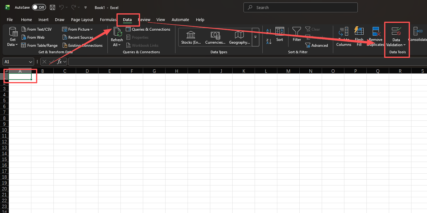
How to Access Data Validation
- Select the cell or range you want to validate
- Go to the Data tab in the ribbon
- Click Data Validation in the Data Tools group
The Data Validation Dialog Box
The dialog box has three tabs:
| Tab | Purpose |
|---|---|
| Settings | Define the validation criteria (type, range, formula) |
| Input Message | Show a tooltip when the cell is selected |
| Error Alert | Customize the error message when invalid data is entered |
2. Creating Drop-Down Lists
Method 1: Direct Input
The simplest way to create a drop-down list is to type the items directly.
- Select the target cells
- Open the Data Validation dialog box
- In the Allow drop-down, select List
- In the Source field, enter items separated by commas, e.g.,
Monday,Tuesday,Wednesday,Thursday,Friday - Click OK
Method 2: Cell Range Reference
For longer lists or lists that may change, reference a range of cells instead.
Suppose you have a list of departments in cells E2:E6:
| Cell | Value |
|---|---|
| E2 | Sales |
| E3 | Marketing |
| E4 | Engineering |
| E5 | Finance |
| E6 | HR |
- Select the target cells (e.g., B2:B20)
- Open Data Validation → List
- In the Source field, select the range
=$E$2:$E$6 - Click OK
Using absolute references ($E$2:$E$6) ensures the source range stays fixed
when copying the validation to other cells.
Method 3: Dynamic Drop-Down with Table
If you format your source data as an Excel Table (Ctrl+T), the drop-down list automatically expands when new items are added.
- Select your source list and press Ctrl+T to create a Table
- In the Data Validation Source field, use the INDIRECT function:
=INDIRECT("Table1[Department]")This way, adding a new department to the table automatically updates all drop-down lists.
3. Limiting Value Ranges
Whole Number and Decimal Validation
Restrict cells to accept only numbers within a specific range.
Suppose you have an order form and want to limit the quantity column to whole numbers between 1 and 500:
- Select the Quantity column cells (e.g., C2:C100)
- Open Data Validation
- Set Allow to Whole number
- Set Data to between
- Set Minimum to
1and Maximum to500
| Order ID | Product | Quantity (1-500) | Unit Price |
|---|---|---|---|
| 1001 | Laptop | 5 | $999.00 |
| 1002 | Mouse | 200 | $29.99 |
| 1003 | Keyboard | 150 | $79.99 |
For decimal values (e.g., discount rates between 0 and 1), select Decimal instead and set the range accordingly.
Date Validation
Restrict cells to accept only dates within a specific period.
For example, to ensure order dates fall within the year 2026:
- Select the date column cells
- Open Data Validation
- Set Allow to Date
- Set Data to between
- Set Start date to
2026/1/1and End date to2026/12/31
Text Length Validation
Limit the number of characters that can be entered in a cell.
For example, to restrict a Product Code field to exactly 8 characters:
- Select the target cells
- Open Data Validation
- Set Allow to Text length
- Set Data to equal to
- Set Length to
8
4. Input Messages and Error Alerts
Input Messages
Input messages appear as tooltips when a validated cell is selected, guiding users on what to enter.
- In the Data Validation dialog, go to the Input Message tab
- Check Show input message when cell is selected
- Enter a Title (e.g., "Quantity") and Input message (e.g., "Enter a whole number between 1 and 500")
Error Alerts
Error alerts appear when invalid data is entered. Excel offers three alert styles:
| Style | Icon | Behavior |
|---|---|---|
| Stop | Red circle with X | Blocks invalid entry completely |
| Warning | Yellow triangle with ! | Warns but allows user to proceed |
| Information | Blue circle with i | Informs but allows entry |
- Go to the Error Alert tab
- Select the Style (Stop, Warning, or Information)
- Enter a Title and Error message
Use Stop for strict rules (e.g., required formats), Warning for soft guidelines, and Information for helpful hints.
5. Custom Validation Rules
Custom validation uses formulas to create rules that go beyond the built-in options. Set Allow to Custom and enter a formula that returns TRUE (valid) or FALSE (invalid).
Common Custom Validation Formulas
| Purpose | Formula | Description |
|---|---|---|
| Unique values only | =COUNTIF($A:$A,A2)=1 |
Prevents duplicate entries in column A |
| Must contain "@" | =ISNUMBER(FIND("@",A2)) |
Basic email format check |
| Text length limit | =LEN(A2)<=10 |
Maximum 10 characters |
| Must start with "PRD-" | =LEFT(A2,4)="PRD-" |
Enforce a prefix pattern |
| No spaces allowed | =LEN(A2)=LEN(SUBSTITUTE(A2," ","")) |
Reject entries containing spaces |
| Future dates only | =A2>TODAY() |
Only allow dates after today |
Example: Preventing Duplicate Employee IDs
Suppose you have an employee list and want to ensure no duplicate IDs are entered:
| Employee ID | Name | Department |
|---|---|---|
| EMP001 | Alice | Sales |
| EMP002 | Bob | Marketing |
| EMP003 | Carol | Engineering |
- Select the Employee ID column (A2:A100)
- Open Data Validation → Custom
- Enter the formula:
=COUNTIF($A:$A,A2)=1 - Set the Error Alert to Stop with the message: "This Employee ID already exists. Please enter a unique ID."
Example: Email Format Validation
To validate that an entry contains both "@" and ".":
=AND(ISNUMBER(FIND("@",A2)), ISNUMBER(FIND(".",A2)), FIND("@",A2)<FIND(".",A2,FIND("@",A2)))This formula checks that the cell contains "@", contains ".", and the "." appears after the "@".
6. Dependent (Cascading) Drop-Down Lists
Dependent drop-downs change their options based on a selection in another cell. For example, selecting a department shows only the job titles for that department.
Step 1: Prepare the Source Data
Create a reference table with departments and their corresponding job titles:
| Sales | Marketing | Engineering |
|---|---|---|
| Account Executive | Content Writer | Software Engineer |
| Sales Manager | SEO Specialist | QA Engineer |
| Sales Rep | Brand Manager | DevOps Engineer |
Step 2: Create Named Ranges
For each department column, create a named range:
- Select cells under "Sales" (e.g., F2:F4)
- Go to Formulas → Define Name
- Name it
Sales(must match the department name exactly) - Repeat for "Marketing" and "Engineering"
Step 3: Set Up the First Drop-Down
Create a regular drop-down list for the Department column (B2) with the values: Sales, Marketing, Engineering.
Step 4: Set Up the Dependent Drop-Down
- Select the Job Title column cells (C2:C100)
- Open Data Validation → List
- In the Source field, enter:
=INDIRECT(B2)
The INDIRECT function converts the text in B2 (e.g., "Sales") into a reference to the named range "Sales", dynamically loading the correct list of job titles.
Important: The named range names must exactly match the values in the first drop-down. If a department name contains spaces (e.g., "Human Resources"), use underscores in the named range (e.g., "Human_Resources") and adjust the formula:
=INDIRECT(SUBSTITUTE(B2," ","_"))7. Tips and Common Operations
Circle Invalid Data
If data was entered before validation rules were applied, you can find existing invalid entries:
- Go to Data → Data Validation → Circle Invalid Data
- Excel will draw red circles around cells that violate the rules
Copy Validation to Other Cells
- Select a cell with the validation rule
- Press Ctrl+C to copy
- Select the target range
- Press Ctrl+Alt+V (Paste Special) → select Validation → OK
Find All Cells with Validation
- Press Ctrl+G (Go To) → Special
- Select Data validation → All
- Click OK — all validated cells will be selected
Remove Validation
- Select the cells with validation
- Open Data Validation dialog
- Click Clear All → OK
Summary
Data validation is an essential tool for maintaining data accuracy in Excel. Through this article, you should have mastered:
- Setting up drop-down lists using direct input, cell references, and dynamic tables
- Restricting value ranges for numbers, dates, and text length
- Creating custom validation rules with formulas
- Building dependent (cascading) drop-down lists with named ranges and INDIRECT
- Configuring input messages and error alerts
- Practical tips for managing validation across your worksheets
By combining these techniques, you can create professional data entry forms that minimize errors and ensure data consistency across your organization.
Was this guide helpful?
If something is missing or unclear, open an issue and we will improve it.
Send feedback