
Excel FILTER Function: Extract Matching Rows
Formula not working?
Share a small sample and the result you expected.
1. Introduction
The FILTER function lets Excel return only the rows or columns that match your criteria. Instead of manually using the worksheet filter buttons, you can write one formula and let the result update automatically when the source data changes.
This is especially useful for dashboards, monthly reports, task lists, sales summaries, and any workbook where you repeatedly need the same filtered view. In this guide, you will learn the syntax, practical examples, multiple criteria patterns, common errors, and when to choose FILTER instead of traditional filtering.
2. FILTER Function Basics
The FILTER function returns a dynamic array. That means the formula can spill results into multiple cells automatically.
=FILTER(array, include, [if_empty])- array: The range you want to return
- include: A TRUE/FALSE test that decides which rows or columns to keep
- if_empty: Optional text or value to show when there are no matches
The most important idea is this: array is what you want back, and include is the condition that chooses the matching records.
Example Data
Suppose you have this order table:
| Date | Region | Product | Status | Amount |
|---|---|---|---|---|
| 2026-01-03 | East | Basic | Paid | 420 |
| 2026-01-05 | West | Pro | Paid | 680 |
| 2026-01-09 | East | Pro | Pending | 750 |
| 2026-01-14 | North | Basic | Paid | 310 |
| 2026-01-18 | East | Pro | Paid | 920 |
| 2026-02-02 | West | Basic | Pending | 260 |
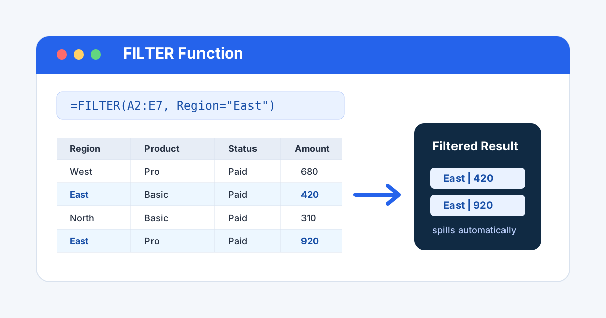
To return all rows where Region is East:
=FILTER(A2:E7,B2:B7="East")The result spills into the cells below and to the right, returning all matching East rows.
3. Add a Friendly Message When No Rows Match
If FILTER finds no matching records, Excel returns a #CALC! error unless you provide the optional if_empty argument.
=FILTER(A2:E7,B2:B7="South","No matching rows")This formula searches for South region orders. If none exist, Excel displays No matching rows instead of an error.
Use this in reports where blank or error-looking results might confuse readers.
4. Filter by a Cell Value
Hard-coded criteria are fine for quick formulas, but dashboard formulas are easier to reuse when the condition lives in a cell.
| Cell | Value |
|---|---|
| H2 | East |
=FILTER(A2:E7,B2:B7=H2,"No matching rows")Now you can change H2 from East to West, North, or another region, and the filtered output updates immediately.
This pattern is useful for report selectors, dropdown-driven summaries, and reusable templates.
5. Filter with Multiple AND Conditions
To keep rows that meet multiple conditions at the same time, multiply the TRUE/FALSE tests. In Excel formulas, TRUE behaves like 1 and FALSE behaves like 0, so multiplication works like AND logic.
To return East region orders where Status is Paid:
=FILTER(A2:E7,(B2:B7="East")*(D2:D7="Paid"),"No matching rows")Result:
| Date | Region | Product | Status | Amount |
|---|---|---|---|---|
| 2026-01-03 | East | Basic | Paid | 420 |
| 2026-01-18 | East | Pro | Paid | 920 |
Each row must pass both tests to appear in the result.
6. Filter with OR Conditions
To keep rows that match any of several conditions, add the TRUE/FALSE tests. Addition works like OR logic because any matching test produces a positive number.
To return orders from East or West:
=FILTER(A2:E7,(B2:B7="East")+(B2:B7="West"),"No matching rows")This keeps rows where Region is East plus rows where Region is West.
You can also combine OR logic with another condition. For example, return paid orders from East or West:
=FILTER(A2:E7,((B2:B7="East")+(B2:B7="West"))*(D2:D7="Paid"),"No matching rows")The extra parentheses matter because they group the OR logic before applying the paid-status condition.
7. Filter Dates Without Hard-Coding the Month
For date-based reports, you can use helper cells or date functions. A simple way to extract January rows is to test the month number.
=FILTER(A2:E7,MONTH(A2:A7)=1,"No January rows")This returns rows where the date falls in January.
If your data covers multiple years, include the year as a second condition:
=FILTER(A2:E7,(MONTH(A2:A7)=1)*(YEAR(A2:A7)=2026),"No January 2026 rows")For recurring reports, place the month and year in cells so users can change the period without editing the formula.
8. Return Only Specific Columns
Sometimes you do not want the full source table. You may only need Product, Status, and Amount. You can combine FILTER with CHOOSECOLS to return selected columns.
=CHOOSECOLS(FILTER(A2:E7,B2:B7="East","No matching rows"),3,4,5)This filters East rows first, then returns only columns 3, 4, and 5 from the filtered result.
Output:
| Product | Status | Amount |
|---|---|---|
| Basic | Paid | 420 |
| Pro | Pending | 750 |
| Pro | Paid | 920 |
This is a clean way to build compact report blocks from wide source tables.
9. Sort Filtered Results
FILTER returns matching rows in the same order as the source data. If you want the output sorted, wrap the formula in SORT.
To return East orders sorted by Amount from largest to smallest:
=SORT(FILTER(A2:E7,B2:B7="East","No matching rows"),5,-1)5sorts by the fifth column of the filtered result-1sorts in descending order
This is great for top-customer lists, open tasks by due date, or sales reports sorted by value.
10. Return a Unique Filtered List
You can combine FILTER with UNIQUE to return a deduplicated list.
To list unique products sold in the East region:
=UNIQUE(FILTER(C2:C7,B2:B7="East","No matching products"))Result:
| Product |
|---|
| Basic |
| Pro |
This pattern is useful for dependent dropdown lists, summary tables, and report controls.
11. Common FILTER Errors
Error 1: #SPILL!
#SPILL! means Excel cannot place the full result on the worksheet. The spill range may be blocked by existing values, merged cells, or another spilled formula.
Fixes:
- Clear the cells where the output needs to spill
- Unmerge cells in the output area
- Move the formula to a blank area of the sheet
For a complete checklist, see Excel #SPILL error causes and fixes.
Error 2: #CALC!
#CALC! often appears when no rows match and the if_empty argument is missing.
=FILTER(A2:E7,B2:B7="South","No matching rows")Adding a friendly fallback message usually solves the problem.
Error 3: Include Range Has the Wrong Size
The include argument must align with the array being filtered. If you filter rows from A2:E7, the include range should usually have the same number of rows.
Correct:
=FILTER(A2:E7,B2:B7="East")Wrong:
=FILTER(A2:E7,B2:B6="East")The second formula checks only five rows while the array contains six rows.
Excel returns #VALUE! for a size mismatch rather than a partial result, which
is the clue that the two ranges need to be resized.
Error 4: FILTER Is Not Available
FILTER is a dynamic array function. It is available in Microsoft 365, Excel for the web, and newer perpetual Excel versions. If a workbook must support older Excel versions, consider Advanced Filter, PivotTables, Power Query, or helper-column formulas instead.
12. FILTER vs Worksheet Filters
Both tools are useful, but they solve different problems.
| Need | Better Choice |
|---|---|
| Quick one-time exploration | Worksheet filter buttons |
| A formula-driven report block | FILTER |
| A dashboard controlled by input cells | FILTER |
| Manual review of a large table | Worksheet filter buttons |
| Reusable extracted lists | FILTER |
Use worksheet filters when you are exploring. Use FILTER when you want the filtered result to become part of a repeatable workbook workflow.
13. Practice Example
Using the sample order table, answer these questions:
| Question | Formula |
|---|---|
| Return all paid orders | =FILTER(A2:E7,D2:D7="Paid","No paid orders") |
| Return all Pro product orders | =FILTER(A2:E7,C2:C7="Pro","No Pro orders") |
| Return East paid orders | =FILTER(A2:E7,(B2:B7="East")*(D2:D7="Paid"),"No matching rows") |
| Return unique products in East | =UNIQUE(FILTER(C2:C7,B2:B7="East","No matching products")) |
Reference answers:
| Question | Expected Result |
|---|---|
| Return all paid orders | 4 rows |
| Return all Pro product orders | 3 rows |
| Return East paid orders | 2 rows |
| Return unique products in East | Basic, Pro |
14. Filter by a List, Partial Text, or a Whole Column
Equality tests cover most reports. These patterns handle what comes next: a list of acceptable values, text that only partly matches, and returning columns instead of rows.
| Goal | Formula |
|---|---|
| Keep rows whose Region is in a short list | =FILTER(A2:E7,ISNUMBER(MATCH(B2:B7,{"East";"North"},0)),"No matching rows") |
| Keep rows whose Product contains "Pro" | =FILTER(A2:E7,ISNUMBER(SEARCH("Pro",C2:C7)),"No matching rows") |
| Use a criteria list stored in cells | =FILTER(A2:E7,ISNUMBER(MATCH(B2:B7,H2:H4,0)),"No matching rows") |
| Drop rows with a blank Amount | =FILTER(A2:E7,D2:D7<>"","No matching rows") |
| Return only the Amount column | =FILTER(A1:E7,A1:E1="Amount","No column found") |
| Exclude one region instead of including several | =FILTER(A2:E7,B2:B7<>"South","No matching rows") |
Three details decide whether these work:
MATCHinsideISNUMBERis the cleanest way to test against a list. WritingB2:B7={"East";"North"}directly only works when the list length matches the range length, which is easy to get wrong.- An array constant uses a semicolon between rows and a comma between columns in
the default en-US setup, and those separators change in other regional
settings. When in doubt, put the values in cells and point
MATCHat them. SEARCHis case-insensitive and returns the position of the match, soISNUMBERturns that position into a usable TRUE or FALSE.FINDdoes the same job but is case-sensitive.
When the include argument is a single row rather than a single column, FILTER
returns columns instead of rows. That is how the Amount-only example above
returns one column from the whole table.
15. Conclusion
The FILTER function is one of the most practical dynamic array tools in Excel. It turns repeated manual filtering into a formula that updates automatically, and it becomes even more powerful when combined with functions like SORT, UNIQUE, and CHOOSECOLS.
Start with one simple condition, add if_empty for cleaner reports, then build up to multiple conditions when your workbook needs more control. Once you understand the include argument, FILTER becomes a reliable way to extract exactly the rows your report needs.
16. Related Guides
- Choose between dynamic row extraction and one-value lookups with Excel FILTER vs VLOOKUP.
- Use Excel dynamic array formulas to understand how spill ranges power
FILTER,SORT, andUNIQUE. - Create missing-value reports with How to Compare Two Columns in Excel.
- Compare filtered rows with criteria-based totals in Excel SUMIF and SUMIFS.
- Choose the right conditional total formula with SUMIF vs SUMIFS in Excel.
- Build row-level logical tests with IF with AND OR in Excel.
- If filtered results keep running into blank edges, review TRIMRANGE and trim references.
- Fix blocked spill ranges with Excel #SPILL error causes and fixes.
Need help fixing a formula?
Share the formula, a small sample table, and the result you expected. This free beta helps us learn which Excel problems readers actually need solved.
Ask for formula help