
Excel Pivot Tables for Beginners: Summarize Data
1. Introduction
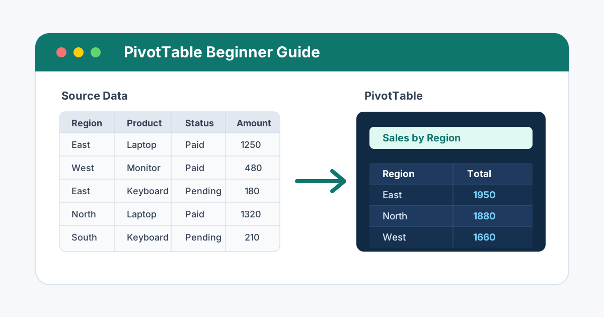
A PivotTable is one of Excel's fastest ways to summarize a list of data. Instead of writing formulas for every question, you can drag fields into a report layout and instantly see totals, counts, averages, and grouped views.
If you have ever asked questions like "Which region sold the most?", "What were monthly sales by product?", or "How many orders are still pending?", a PivotTable is often the cleanest first tool to try.
In this tutorial, you will create a beginner-friendly sales report from a small table, learn what Rows, Columns, Values, and Filters actually do, and fix the mistakes that usually trip up first-time PivotTable users.
2. Prepare Source Data
PivotTables work best when your source data is a clean list. Each column should have a clear header, each row should be one record, and there should be no blank rows inside the dataset.
Use this sample data to follow along:
| Order Date | Region | Product | Sales Rep | Status | Amount |
|---|---|---|---|---|---|
| 2026-01-03 | East | Laptop | Mia | Paid | 1250 |
| 2026-01-06 | West | Monitor | Leo | Paid | 480 |
| 2026-01-11 | East | Keyboard | Mia | Pending | 180 |
| 2026-01-18 | North | Laptop | Ava | Paid | 1320 |
| 2026-02-02 | West | Laptop | Leo | Paid | 1180 |
| 2026-02-08 | East | Monitor | Noah | Paid | 520 |
| 2026-02-14 | South | Keyboard | Ava | Pending | 210 |
| 2026-02-22 | North | Monitor | Noah | Paid | 560 |
Before inserting a PivotTable, check these basics:
- Every column has a header
- There are no completely blank rows or columns inside the list
- Dates are real dates, not text that only looks like dates
- Amount values are numbers, not numbers stored as text
- Similar labels are consistent, such as
Eastinstead of bothEastandE.
If your data is messy, clean it first. The guides on Excel Data Cleaning and Excel Data Sorting are good companions before building a report.
3. Insert Your First PivotTable
To create a PivotTable from the sample data:
- Click any cell inside the source data.
- Go to Insert, then choose PivotTable.
- Confirm the selected table or range.
- Choose New Worksheet for a clean report area.
- Click OK.
Excel creates an empty PivotTable area and opens the PivotTable Fields pane. This pane is where you build the report by dragging field names into four areas: Rows, Columns, Values, and Filters.
For your first report, drag:
| Field | Drop Area |
|---|---|
| Region | Rows |
| Amount | Values |
Excel should now show total sales by region.
| Region | Sum of Amount |
|---|---|
| East | 1950 |
| North | 1880 |
| South | 210 |
| West | 1660 |
| Grand Total | 5700 |
That is the basic PivotTable idea: choose a category, choose a number, and Excel calculates the summary.
4. Understand Rows, Columns, Values, and Filters
The four PivotTable areas control the report layout.
| Area | What It Does | Example |
|---|---|---|
| Rows | Groups records vertically | Region, Product, Sales Rep |
| Columns | Groups records horizontally | Month, Status, Product |
| Values | Calculates numbers | Sum of Amount, Count of Orders |
| Filters | Adds a report-level filter | Status, Region, Sales Rep |
Here is a practical way to think about it:
- Put the question's main category in Rows.
- Put the number you want to summarize in Values.
- Put a second comparison category in Columns.
- Put optional slicer-style controls in Filters.
For example, to see sales by region and product:
| Field | Drop Area |
|---|---|
| Region | Rows |
| Product | Columns |
| Amount | Values |
The PivotTable will show a cross-tab report like this:
| Region | Keyboard | Laptop | Monitor | Grand Total |
|---|---|---|---|---|
| East | 180 | 1250 | 520 | 1950 |
| North | 0 | 1320 | 560 | 1880 |
| South | 210 | 0 | 0 | 210 |
| West | 0 | 1180 | 480 | 1660 |
| Grand Total | 390 | 3750 | 1560 | 5700 |
5. Change Sum to Count or Average
When you drop a numeric field into Values, Excel usually summarizes it with Sum. You can change the calculation.
To change the summary type:
- Click any number in the PivotTable values area.
- Right-click and choose Summarize Values By.
- Choose Sum, Count, Average, Max, or Min.
Common choices:
| Summary Type | Use It When You Need |
|---|---|
| Sum | Total sales, total cost, total quantity |
| Count | Number of orders, tickets, tasks, or records |
| Average | Average order value, average score, average time |
| Max | Highest sale, latest score, largest amount |
| Min | Lowest sale, smallest amount, earliest value |
For example, if you change Amount from Sum to Average, the report answers "What is the average order amount by region?" instead of "What is total sales by region?"
6. Add a Report Filter
Filters let you narrow the whole PivotTable without changing the source data.
To filter the report to paid orders only:
- Drag
Statusto the Filters area. - Open the filter dropdown at the top of the PivotTable.
- Choose
Paid.
Now the PivotTable ignores pending orders and summarizes only paid records.
| Region | Sum of Amount for Paid Orders |
|---|---|
| East | 1770 |
| North | 1880 |
| West | 1660 |
| Grand Total | 5310 |
Filters are useful for quick reports, but if you want a more interactive dashboard, Excel slicers are often easier for readers to use. That is a good next step after you are comfortable with basic PivotTables.
7. Group Dates by Month
Date grouping is one of the most useful PivotTable features for sales and operations reports.
To summarize sales by month:
- Drag
Order Dateto Rows. - Drag
Amountto Values. - Right-click one of the dates in the PivotTable.
- Choose Group.
- Select Months, then click OK.
Your report becomes a monthly summary:
| Month | Sum of Amount |
|---|---|
| Jan | 3230 |
| Feb | 2470 |
| Grand Total | 5700 |
If date grouping does not work, the source date column probably contains text, blanks, or invalid dates. Clean the date column first, then refresh the PivotTable.
8. Refresh a PivotTable
A PivotTable does not always update automatically when source data changes. If you edit the source table, add rows, or fix values, refresh the PivotTable.
To refresh:
- Click inside the PivotTable.
- Right-click and choose Refresh.
If you add new rows below the original data range, Excel may not include them unless the source range expands. A simple best practice is to convert the source data into an Excel Table before creating the PivotTable.
To create an Excel Table:
- Click inside the source data.
- Press Ctrl+T.
- Confirm that My table has headers is checked.
- Click OK.
When a PivotTable is based on an Excel Table, new rows added to the table are easier to include after refresh.
9. Format PivotTable Values
Raw numbers are harder to scan. For sales reports, format Amount as currency or number with separators.
To format values:
- Right-click any value in the PivotTable.
- Choose Value Field Settings.
- Click Number Format.
- Choose Currency, Accounting, or Number.
- Click OK twice.
This formatting stays with the PivotTable field better than formatting random worksheet cells around the report.
You can also rename fields. For example, change Sum of Amount to Total Sales so the report reads more naturally.
10. Common Beginner Mistakes
Mistake 1: Blank Headers
PivotTables need field names. If a source column has no header, Excel cannot build the field list correctly.
Fix: Add a short, clear header to every column before creating the PivotTable.
Mistake 2: Blank Rows Inside the Data
Blank rows can make Excel select only part of the dataset.
Fix: Remove blank rows or convert the whole data range into an Excel Table.
Mistake 3: Numbers Stored as Text
If Amount values are stored as text, Excel may count them instead of summing them.
Fix: Convert the Amount column to real numbers before building the report.
Mistake 4: Expecting New Data to Appear Automatically
PivotTables usually need a refresh after source data changes.
Fix: Right-click the PivotTable and choose Refresh. If new rows are missing, check the source range.
Mistake 5: Too Many Fields at Once
Adding many fields can create a crowded report that is hard to read.
Fix: Start with one row field and one value field. Add columns, filters, or extra row levels only when they answer a real question.
For advanced display issues, especially error values in calculated fields, see the deeper guide on PivotTable error value display.
11. PivotTables vs Formulas vs FILTER
PivotTables, formulas, and dynamic array functions can all summarize data, but each has a different strength.
| Need | Better Choice |
|---|---|
| Explore a dataset quickly | PivotTable |
| Build a reusable dashboard number | Formula |
| Extract matching detail rows | FILTER |
| Group dates and compare categories | PivotTable |
| Create a custom calculation layout | Formula |
Use a PivotTable when you want to explore and summarize. Use formulas when you need exact custom logic in fixed cells. Use FILTER when you need the matching rows themselves, not just a summary.
12. Practice Exercise
Using the sample sales table, build these PivotTables:
| Task | Fields to Use |
|---|---|
| Total sales by region | Region in Rows, Amount in Values |
| Total sales by product | Product in Rows, Amount in Values |
| Paid orders by region | Region in Rows, Amount in Values, Status in Filters |
| Monthly sales | Order Date in Rows grouped by Month, Amount in Values |
Reference answers:
| Question | Expected Result |
|---|---|
| Total sales by region | East 1950, North 1880, South 210, West 1660 |
| Total sales by product | Keyboard 390, Laptop 3750, Monitor 1560 |
| Paid sales total | 5310 |
| Monthly sales | Jan 3230, Feb 2470 |
Conclusion
PivotTables help you turn a raw list into a useful summary without writing formulas. Start with clean source data, place one category in Rows, place a numeric field in Values, and then add Columns or Filters only when they make the report clearer.
Once you are comfortable with the basics, the next skills to learn are grouping dates, adding slicers, changing value calculations, and formatting reports so other people can read them quickly.
Was this guide helpful?
If something is missing or unclear, open an issue and we will improve it.
Send feedback