Excel PivotTable Error Value Display Mechanism Analysis

Excel PivotTables employ specific error handling mechanisms that differ between native aggregation and custom calculated fields. This technical analysis explains why the "For error values show" setting appears to fail for calculated fields and provides solutions based on Excel's internal processing logic.

Problem Phenomenon Description

Here's a common scenario: You've created a PivotTable with calculated fields, and some results return #DIV/0! errors. You follow the standard procedure:

1. Right-click the data area → Select "PivotTable Options"
2. In the "Layout & Format" tab, check "For error values show"
3. Type "-" and click OK

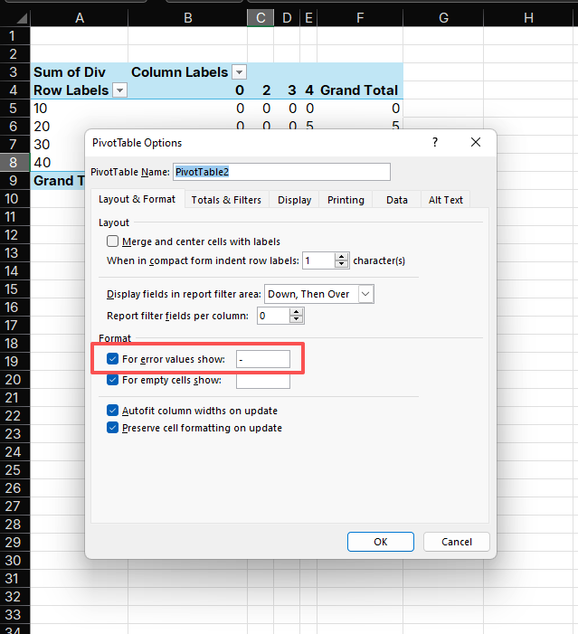
But the result still shows 0. This confuses many users, who often think it's an Excel glitch. The truth? This is maybe a deliberate design decision by Microsoft's Excel team.

Hypothesis on the Root Cause

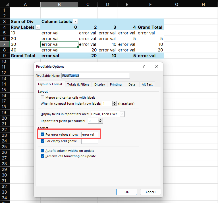
In many formula calculations, the hyphen (-) is used to indicate no result or a zero value. This convention might explain why Excel PivotTable's error value strategy for calculated fields converts '-' to 0. Currently, there is insufficient evidence to validate this hypothesis, however PivotTable will display any configured string except '-' as literal text.

Comparative Analysis with Google Sheets

Google Sheets implements error handling through explicit formula logic rather than interface settings:

=IFERROR(Sales/Quantity, "-")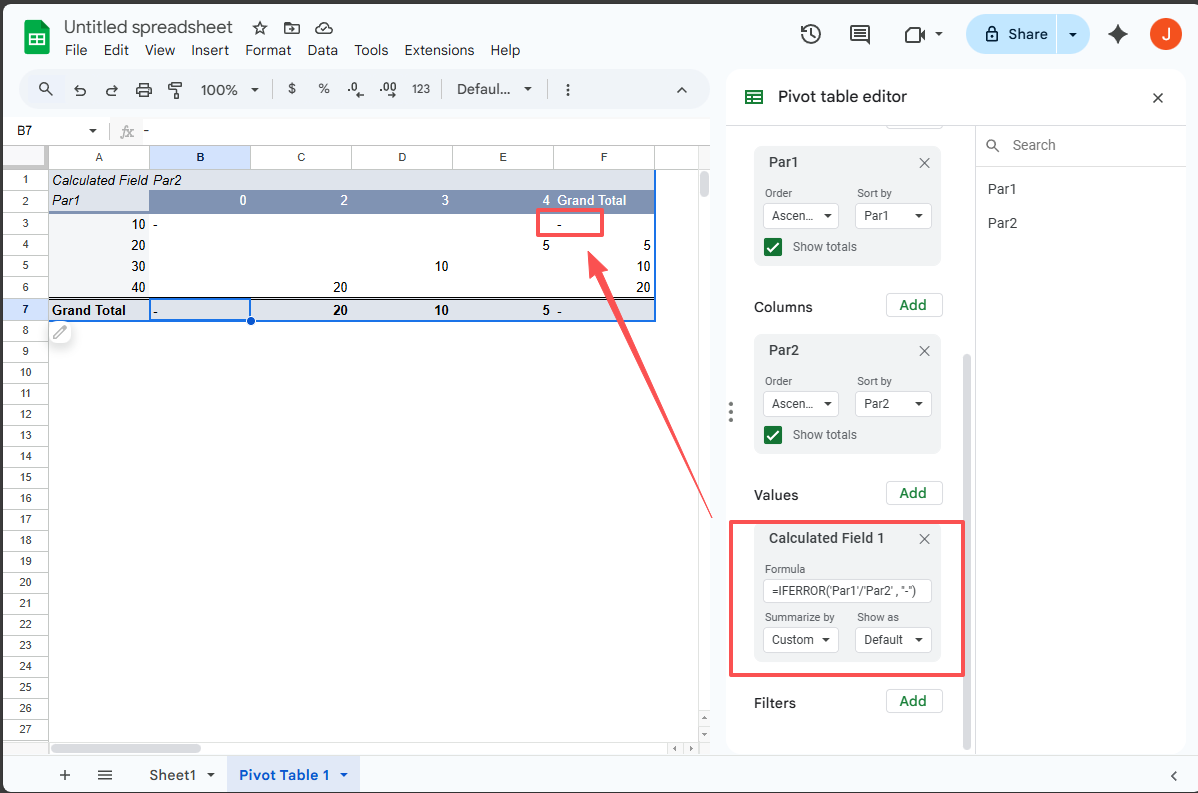

This implementation difference stems from distinct design:

• Excel: Provides an error value display mechanism based on formatting settings, suitable for native aggregated fields.
• Google Sheets: Allows users to solve problems within formulas.

The Simple Solution

The solution requires understanding Excel's formatting precedence. The technical implementation principle is:

For calculated fields, custom number formatting takes priority over PivotTable error value settings

Step-by-step solution:

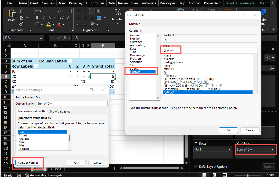
1. Select the calculated field's Value Field Settings to open dialog.
2. Click "Format Cells" (or press Ctrl+1) to open Format Cells, select "Custom"
3. Enter this format code: 0;-0;-;@
   • Positive numbers show as digits
   • Negative numbers show with minus signs
   • Errors display as "-"
   • Text appears normally

Conclusion

Excel's PivotTable error display behavior for calculated fields represents an intentional design choice that prioritizes calculation transparency over surface-level presentation. The custom number format solution presented enables users to achieve the desired error visualization without compromising formula integrity or calculation accuracy.

This analysis underscores the importance of understanding Excel's internal processing mechanisms when working with advanced PivotTable features, particularly when dealing with calculated fields and error value presentation.