How to Merge Cells in Excel Without Losing Data (Step-by-Step)​

If you’ve ever tried to merge cells in Excel, you might have hit a frustrating roadblock: Excel’s default “Merge & Center” button often deletes data from all cells except the top-left one. This is a nightmare when you need to combine text from multiple cells (like first names and last names in separate columns) or keep all information while creating a clean header.​

The good news? You don’t have to choose between merged cells and lost data. Below is a simple, beginner-friendly guide to merging cells in Excel without deleting any content—works for Excel 2019, 2021, 365, and even older versions.​

What You’ll Need Before Starting​

• A basic Excel workbook with data you want to merge (e.g., cells A1, B1, and C1 with different text).​
• No advanced skills required—we’ll use built-in Excel tools, no formulas needed (though we’ll share a formula trick too!).​

Method 1: Use “Merge Across” or “Merge Cells” (For Headers, No Data Loss)​

This method is best when you want to merge cells for formatting (like a table header) and only have data in the top-left cell (the rest are empty). It’s the safest way to avoid accidental data loss.​

Step 1: Select the cells you want to merge​

Click and drag your mouse to highlight the cells. For example, if you want to merge A1, B1, and C1 into one header cell, select all three.​ ​

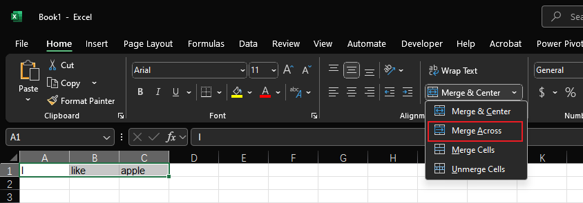
Step 2: Choose the right “Merge” option (not “Merge & Center”)​

Go to the Home tab in the Excel ribbon. Look for the “Alignment” group (it’s usually on the right side of the ribbon).​

Instead of clicking the big “Merge & Center” button (which deletes extra data), click the small dropdown arrow next to it to open the merge menu.​

From the menu, select one of these two options:​

• Merge Across: Merges cells in the same row (e.g., A1-C1) into one horizontal cell.​
• Merge Cells: Merges cells in any selection (rows or columns) into one cell.​

Avoid “Merge & Center” here unless you’re sure only the top-left cell has data!​ ​ ​

Step 3: Confirm the merge (if prompted)​

If Excel detects data in more than one cell, it will pop up a warning: “Merging cells only keeps the data in the upper-left cell of the range.”​

• If you only have data in the top-left cell (the rest are empty), click “OK”—your cells will merge, and no data will be lost.​
• If you have data in multiple cells, stop here! Use Method 2 instead (we’ll show you how to keep all data).​

Method 2: Combine Data from Multiple Cells First (No Data Loss)​

If you have data in all cells you want to merge (e.g., A1 = “I”, B1 = “like”, C1 = “Apple”), you need to first combine the data into one cell—then merge the rest. Here’s how:​

Step 1: Combine data with the CONCATENATE function (or “&” symbol)​

Insert a new empty cell next to your data (e.g., if your data is in A1-C1, use D1 as the “combined cell”).​

In the empty cell, type one of these two formulas (they do the same thing—pick whichever is easier to remember):​

• Using CONCATENATE: =CONCATENATE(A1, " ", B1, " ", C1)​ (The " " adds a space between each cell’s data—replace with a comma, hyphen, or nothing if you want.)​
• Using “&” (simpler): =A1 & " " & B1 & " " & C1​ Press Enter. The empty cell will now show the combined data (e.g., “I like Apple”).​

  

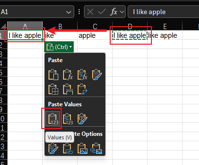
Step 2: Copy the combined data (so it’s not a formula)​

Right-click the cell with the combined data (e.g., D1) and select Copy (or press Ctrl+C on Windows / Cmd+C on Mac).​

Then, right-click the same cell again and select Paste Special > Values (this turns the formula into plain text, so it won’t break if you delete the original cells).​​ ​

Step 3: Merge the original cells (now empty!)​

Delete the data from your original cells (A1-C1) so they’re empty. Then follow Method 1: select A1-C1, use “Merge Across” or “Merge Cells”, and click “OK”.​

Finally, cut (Ctrl+X / Cmd+X) the combined data from D1 and paste it into the merged A1 cell. Done! You now have merged cells with all your original data.​

Bonus: For Google Sheets Users (Quick Comparison)​

If you switch between Excel and Google Sheets, the process is similar—but Google Sheets has a handy “Merge cells” option that lets you keep data by default:​

1. Select cells to merge.​
2. Go to Format > Merge cells.​
3. Choose “Merge all” or “Merge horizontally”—Google Sheets will automatically combine text from all cells (no formula needed!).​

This is one of the few places Google Sheets is simpler than Excel—but our Excel methods above work every time, even if you don’t have a Google account.​

Common Mistakes to Avoid​

1. Using “Merge & Center” with multiple data cells: This is the #1 cause of data loss. Always check the merge dropdown first.​
2. Forgetting to paste as values: If you skip Step 2 in Method 2, deleting the original cells will break your formula (you’ll see #REF! instead of your data).​
3. Merging cells in tables: Excel tables don’t support merged cells—convert your table to a regular range first (right-click the table > “Convert to Range”).​

Final Tip: When to Avoid Merged Cells Altogether​

Merged cells can cause headaches if you later sort or filter your data (Excel might misinterpret merged ranges). If you’re working with a dataset you’ll edit often, try these alternatives:​

• Use “Center Across Selection” (in the Alignment group’s dropdown) to look like merged cells, but keep cells separate.​
• Use the CONCATENATE formula to combine data without merging cells.​

But for headers, titles, or one-time formatting, merged cells are perfectly safe—just use the methods above to keep your data intact!​