Excel AVERAGE Function: Multiple Ways to Calculate Averages
Introduction
The average is one of the most commonly used statistical indicators in data analysis, used to measure the central tendency of data. Excel provides multiple functions for calculating averages, with the AVERAGE function being the most basic and commonly used. This article will detail the various uses of the AVERAGE function family, including basic averages, weighted averages, and averages that exclude error values, helping you choose the appropriate average calculation method for different scenarios.
1. AVERAGE Function Basics
What is the AVERAGE Function?
The AVERAGE function is used to calculate the arithmetic mean of a set of values, which is the sum divided by the number of values.
Syntax
=AVERAGE(number1, [number2], ...)- number1: Required parameter, representing the first value or range of values to average
- number2, ...: Optional parameters, up to 255 values or ranges of values
How to Use Basic AVERAGE
- Select the cell where you want to display the result
- Enter
=AVERAGE( - Select the range of cells you want to average, or enter specific values
- Press Enter to complete
Example
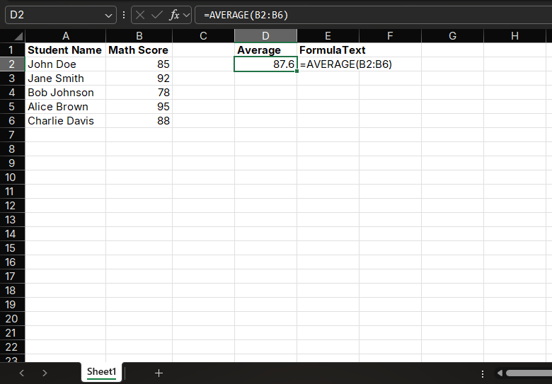
Suppose we have the following student score data:
| Student Name | Math Score |
|---|---|
| John Doe | 85 |
| Jane Smith | 92 |
| Bob Johnson | 78 |
| Alice Brown | 95 |
| Charlie Davis | 88 |
To calculate the average math score, simply enter in a cell:
=AVERAGE(B2:B6)The result will display as 87.6.
Use Cases
- Calculate class average scores
- Statistics monthly average sales
- Calculate average product costs
2. Advanced Uses of the AVERAGE Function
Multi-Range Averaging
The AVERAGE function can calculate averages for multiple non-contiguous ranges simultaneously.
Syntax
=AVERAGE(range1, range2, ...)Example
If you need to calculate the average scores for both Class 1 and Class 2, and these data are in different ranges, you can use:
=AVERAGE(B2:B10, D2:D10)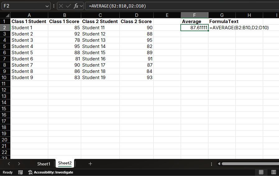
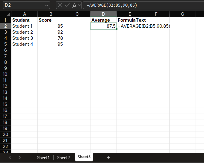
Averaging with Constants
In addition to referencing cell ranges, the AVERAGE function can also use constant values directly.
Example
=AVERAGE(B2:B5, 90, 85)This formula will calculate the average of the range B2:B5, then add 90 and 85 and recalculate the average.
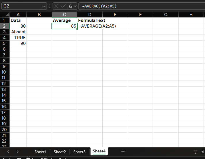
Ignoring Non-Numeric Values
When the argument range of the AVERAGE function contains text, logical values, or blank cells, it automatically ignores these non-numeric values and only calculates the average of numeric values.
Example
If range A1:A4 contains the value 80, the text "Absent", the logical value TRUE,
and the value 90, the formula =AVERAGE(A1:A4) will return 85.
3. AVERAGEA Function: Averages Including Logical Values
What is AVERAGEA?
The AVERAGEA function is used to calculate the average of a set of values. Unlike AVERAGE, it includes logical values and text in the calculation:
- TRUE is treated as 1
- FALSE is treated as 0
- Text values are treated as 0
Syntax
=AVERAGEA(value1, [value2], ...)Example
Using the same data as in the previous section:
If range A1:A4 contains the value 80, the text "Absent", the logical value TRUE,
and the value 90, the formula =AVERAGEA(A1:A4) will return:
(80 + 0 + 1 + 90) / 4 = 42.75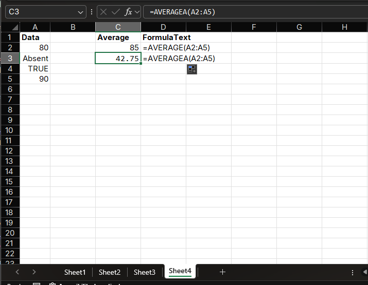
Use Cases
- Calculate class average scores including absent records
- Statistics average values of data containing logical values
4. AVERAGEIF Function: Conditional Averages
What is AVERAGEIF?
The AVERAGEIF function is used to calculate the average of values in a specified range based on a given condition.
Syntax
=AVERAGEIF(range, criteria, [average_range])- range: Required parameter, representing the range of cells to be evaluated based on the condition
- criteria: Required parameter, representing the condition, which can be a number, text, or expression
- average_range: Optional parameter, representing the actual range of cells to average
How to Use
- Select the cell where you want to display the result
- Enter
=AVERAGEIF( - Select the criteria range
- Enter the criteria (text or expression enclosed in quotes)
- Select the range to average (optional)
- Press Enter to complete
Example
Suppose we have the following sales data:
| Product | Sales Revenue |
|---|---|
| A | 1000 |
| B | 1500 |
| A | 1200 |
| C | 800 |
| B | 1300 |
| A | 1100 |
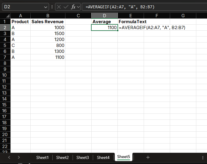
To calculate the average sales revenue for Product A, you can use:
=AVERAGEIF(A2:A7, "A", B2:B7)The result will display as 1100.
Use Cases
- Calculate average sales for specific products
- Statistics average salaries for specific departments
- Calculate average order amounts for specific months
5. AVERAGEIFS Function: Multi-Conditional Averages
What is AVERAGEIFS?
The AVERAGEIFS function is used to calculate the average of values in a specified range based on multiple conditions and is an extended version of the AVERAGEIF function.
Syntax
=AVERAGEIFS(average_range, criteria_range1, criteria1, [criteria_range2, criteria2], ...)- average_range: Required parameter, representing the actual range of cells to average
- criteria_range1: Required parameter, representing the first range of cells to be evaluated based on the condition
- criteria1: Required parameter, representing the first condition
- criteria_range2, criteria2, ...: Optional parameters, up to 127 condition ranges and conditions
Example
Suppose we have the following sales data:
| Product | Region | Sales Revenue |
|---|---|---|
| A | North | 1000 |
| B | South | 1500 |
| A | North | 1200 |
| C | East | 800 |
| B | North | 1300 |
| A | South | 1100 |
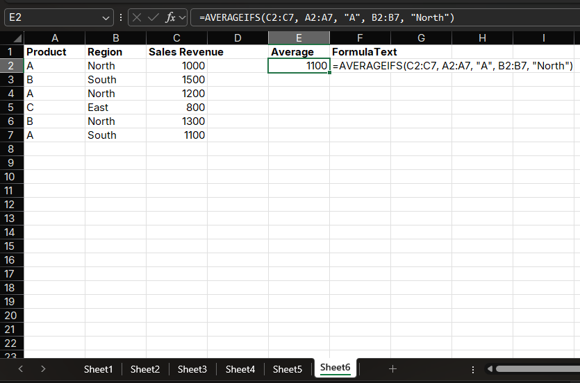
To calculate the average sales revenue for Product A in the North region, you can use:
=AVERAGEIFS(C2:C7, A2:A7, "A", B2:B7, "North")The result will display as 1100.
Use Cases
- Calculate average sales for specific products in specific regions
- Statistics average expenses for specific departments in specific months
- Calculate average income for specific age groups
6. Weighted Average Calculation
What is Weighted Average?
A weighted average is an average that considers the weight of each value, calculated as: (value1×weight1 + value2×weight2 + ...) / total weight
How to Calculate in Excel
Excel does not have a dedicated weighted average function, but you can use a combination of SUMPRODUCT and SUM functions to calculate it.
Syntax
=SUMPRODUCT(numeric_range, weight_range) / SUM(weight_range)Example
Suppose we have the following course scores, where the final exam accounts for 60% and the usual grade accounts for 40%:
| Student Name | Usual Grade | Final Exam |
|---|---|---|
| John Doe | 90 | 85 |
| Jane Smith | 85 | 92 |
| Bob Johnson | 95 | 78 |
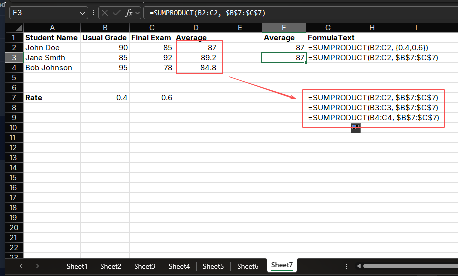
To calculate John Doe's weighted average score, you can use:
=SUMPRODUCT(B2:C2, {0.4, 0.6})Or a more general form:
=SUMPRODUCT(B2:C2, $E$1:$F$1) // Assuming E1=0.4, F1=0.6The result will display as 87.
Use Cases
- Calculate weighted average course scores
- Statistics weighted average product costs
- Calculate weighted average returns for investment portfolios
7. Averages Excluding Error Values
What if There are Errors in Data?
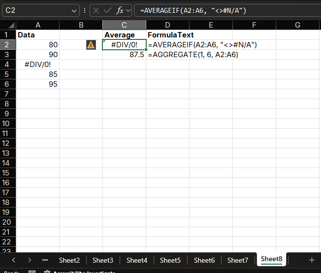
When data contains error values (such as #DIV/0!, #VALUE!, etc.), directly using the AVERAGE function will return an error. In this case, you can use the AVERAGEIF function or the AGGREGATE function to exclude error values.
Method 1: Using AVERAGEIF
=AVERAGEIF(range, "<>#N/A")Method 2: Using AGGREGATE
=AGGREGATE(1, 6, range)- 1 represents average
- 6 represents ignore error values
Example
If range A1:A5 contains the values 80, 90, #DIV/0!, 85, and 95, the formula
=AGGREGATE(1, 6, A1:A5) will return 87.5.
8. Practical Application Examples
Example 1: Grade Point Average (GPA) Calculation
Calculate student GPA, where different courses have different credit weights:
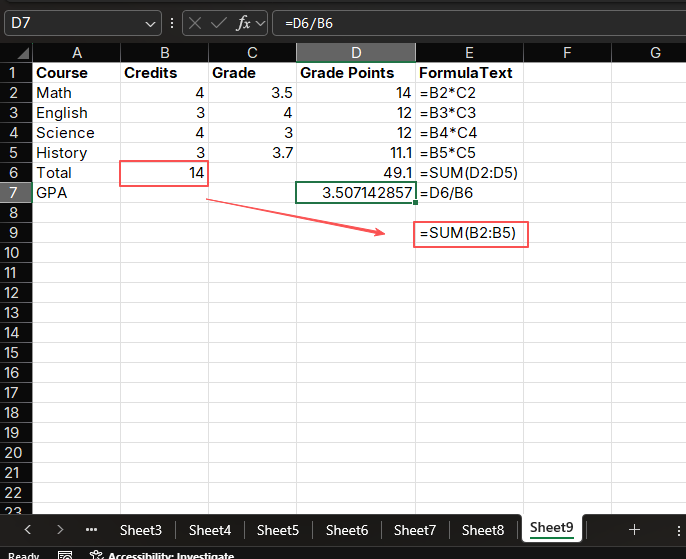
Enter the formula in cell D2:
=B2*C2Copy the formula down to all course rows
Enter the formula in cell B6 to calculate total credits:
=SUM(B2:B5)Enter the formula in cell D6 to calculate total grade points:
=SUM(D2:D5)Enter the formula in cell D8 to calculate GPA:
=D6/B6
Example 2: Monthly Average Temperature
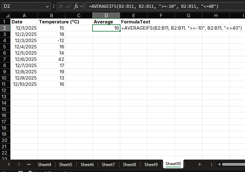
Calculate monthly average temperature, excluding outliers (such as temperatures below -10°C or above 40°C):
- Enter the formula in cell C2:
=AVERAGEIFS(B2:B32, B2:B32, ">=-10", B2:B32, "<=40")
The result will display the monthly average temperature excluding outliers.
Summary
Excel provides multiple functions for calculating averages, from basic AVERAGE to complex AVERAGEIFS, and weighted average calculations, which can meet various data analysis needs. Through this article, you should have mastered:
- Basic usage and advanced applications of the AVERAGE function
- Using AVERAGEIF for single-conditional average calculations
- Using AVERAGEIFS for multi-conditional average calculations
- Methods for calculating weighted averages
- Calculating averages that exclude error values
By proficiently using these functions, you will be able to analyze data more accurately, extract valuable information, and provide support for decision-making.
Have a problem with Excel or Google Sheets?
Tell us about the issue you're facing, and we'll create a step-by-step guide for it.